Over the last two weeks I have been looking at the analysis of the epilespy trial data taken from Thall and Vail (1990). So far I have concentrated on a Bayesian analysis of those data using Stata alone, but this model involves Poisson regression with two random effects, so it is quite complex and it takes a long time to run in Stata. Last week I improved the efficiency of the Stata code and I was able to reduce the run time to 6 minutes but that is still quite slow so perhaps we should to switch to either Mata or WinBUGS for the computation while continuing to use Stata to control the analysis. This week I will consider calling WinBUGS/OpenBUGS/JAGS and in a future posting I will try using Mata.
If you have not followed the discussion of this example it would be sensible to start with the first posting in this series and to read them in order. Click here to link to the first posting in the series.
WinBUGS
I would normally choose only one of WinBUGS/OpenBUGS/JAGS and my preference is for OpenBUGS, but it is sometimes instructive to compare the three, so I will try each in turn starting with WinBUGS.
The Stata code for setting up the problem, calling WinBUGS and reading the results is fairly routine and this simple example presents few problems. I’ll list the code and then say a few words about the structure.
use epilepsy.dta , clear
gen LB = log(Base/4)
qui su LB
gen cLB = LB – r(mean)
gen lnAge = log(Age)
qui su lnAge
gen clnAge = lnAge – r(mean)
gen BXT = LB*Trt
qui su BXT
qui gen cBXT = BXT – r(mean)
qui su Trt
gen cTrt = Trt – r(mean)
wbsmodel EpilepsyWinBUGS.do model.txt
/*
model
{
for(j in 1 : 59) {
for(k in 1 : 4) {
log(mu[j, k]) + aTrt * cTrt[j]
+ aBXT * cBXT[j]
+ aAge * clnAge[j]
+ aV4 * V4[k]
+ u[j] + e[j, k]
y[j, k] ~ dpois(mu[j, k])
e[j, k] ~ dnorm(0.0, taue)
}
u[j] ~ dnorm(0.0, tauu)
}
# priors:
a0 ~ dnorm(2.6,1.0)
aBase ~ dnorm(1.0,1.0)
aTrt ~ dnorm(0.0,1.0)
aBXT ~ dnorm(0.0,1.0)
aAge ~ dnorm(0.0,1.0)
aV4 ~ dnorm(0.0,1.0)
tauu ~ dgamma(8.0,2.0)
taue ~ dgamma(8.0,2.0)
}
*/
wbslist (var cLB cTrt cBXT clnAge) (V4=c(0,0,0,1)) ///
(struct y_1 y_2 y_3 y_4, name(y)) using data.txt , replace
wbslist (a0=2.6, aBase=0, aTrt=0, aBXT=0, aAge=0, aV4=0, tauu=1, taue=1) ///
using init.txt , replace
wbsscript using script.txt, replace ///
model(model.txt) data(data.txt) init(init.txt) log(log.txt) ///
set(a0 aBase aTrt aBXT aAge aV4 tauu taue) ///
burn(5000) update(50000) thin(5) coda(epi)
wbsrun using script.txt, time
type log.txt
wbscoda using epi , clear
gen sigmau = 1/sqrt(tauu)
gen sigmae = 1/sqrt(taue)
mcmcstats a0 aBase aTrt aBXT aAge aV4 sigmau sigmae
mcmctrace a0 aBase aTrt aBXT aAge aV4 sigmau sigmae
The first block reads the data into Stata and centres it. Then the WinBUGS program is written to the file model.txt using the wbsmodel command, which reads the WinBUGS syntax commands that are included as a comment and which are highlighted here in green. The data and initial values files are created as list structures using wbslist, then the script file is created using wbsscript. The script is run using wbsrun and the results are read into Stata using wbscoda. Finally I produce a summary table of the results and draw the trace or history plots using mcmcstats and mcmctrace.
For anyone who has used WinBUGS this is such a straightforward example that there is little left to say. If you have not used WinBUGS before then you can read about WinBUGS in the online manual that comes with the program or you could read about WinBUGS and the wbs Stata commands in Chapter 8 of Bayesian analysis with Stata.
The program takes about 2.25 minutes to run compared with 6 minutes for the pure Stata code that I wrote last week. The results are very similar,
----------------------------------------------------------------------------
Parameter         n     mean       sd     sem   median         95% CrI
----------------------------------------------------------------------------
a0           10000    1.595   0.082   0.0018    1.596 (  1.436,   1.754 )
aBase        10000    0.911   0.129   0.0048    0.911 (  0.660,   1.163 )
aTrt         10000   -0.802   0.368   0.0193   -0.797 ( -1.515,  -0.084 )
aBXT         10000    0.276   0.186   0.0139    0.277 ( -0.089,   0.636 )
aAge         10000    0.393   0.339   0.0069    0.395 ( -0.282,   1.045 )
aV4          10000   -0.098   0.092   0.0011   -0.098 ( -0.277,   0.078 )
sigmau       10000    0.494   0.055   0.0006    0.491 (  0.397,   0.612 )
sigmae       10000    0.407   0.036   0.0005    0.405 (  0.342,   0.486 )
----------------------------------------------------------------------------
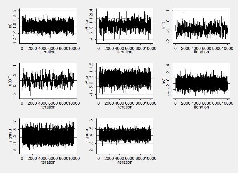
The posterior means only vary from those obtained with Stata alone due to the Monte Carlo nature of the algorithm but WinBUGS gives smaller standard errors indicating better mixing. For instance, the sem of aTrt has dropped from 0.0225 to 0.0193 and the sem of ABase has dropped from 0.0087 to 0.0048. Perhaps Stata’s sems are around 30% worse suggesting that we would need to have run the Stata program for around 1.3^2=1.69 times as long to get the same accuracy. A fair comparison would therefore be 2.25 minutes for WinBUGS and about 10 minutes for the Stata only program.
The improvement in mixing can also be seen by comapring the trace plot below with that given in last week’s posting.
Finally notice the time option on wbsrun that enabled me to tell how long WinBUGS took to run the 55,000 updates. This is an undocumented but useful option. Why is it undocumented? because I forgot to document it. I’ll modify wbsrun.shlp when I release a new version of the wbs programs.
OpenBUGS
The Stata program for calling OpenBUGS is almost identical to that given above for WinBUGS. The only differences are that we must add the openbugs option to wbsscript, wbsrun and wbscoda. The OpenBUGS syntax for this model is identical to the WinBUGS syntax. OpenBUGS is a little quicker than WinBUGS for this problem and takes only 1.5 minutes compared with 2.25 minutes. More importantly OpenBUGS produces a sampler that mixes noticeably better. Here are the results,
----------------------------------------------------------------------------
Parameter         n     mean       sd     sem   median         95% CrI
----------------------------------------------------------------------------
a0           10000    1.594   0.081   0.0014   1.594 (  1.432,   1.752 )
aBase        10000    0.920   0.132   0.0029   0.919 (  0.664,   1.183 )
aTrt         10000   -0.780   0.377   0.0068  -0.780 ( -1.521,  -0.041 )
aBXT         10000    0.262   0.193   0.0045   0.264 ( -0.123,   0.641 )
aAge         10000    0.398   0.343   0.0064   0.393 ( -0.270,   1.071 )
aV4          10000   -0.100   0.092   0.0011  -0.101 ( -0.278,   0.083 )
sigmau       10000    0.495   0.055   0.0006   0.491 (  0.397,   0.612 )
sigmae       10000    0.407   0.036   0.0005   0.405 (  0.340,   0.482 )
----------------------------------------------------------------------------
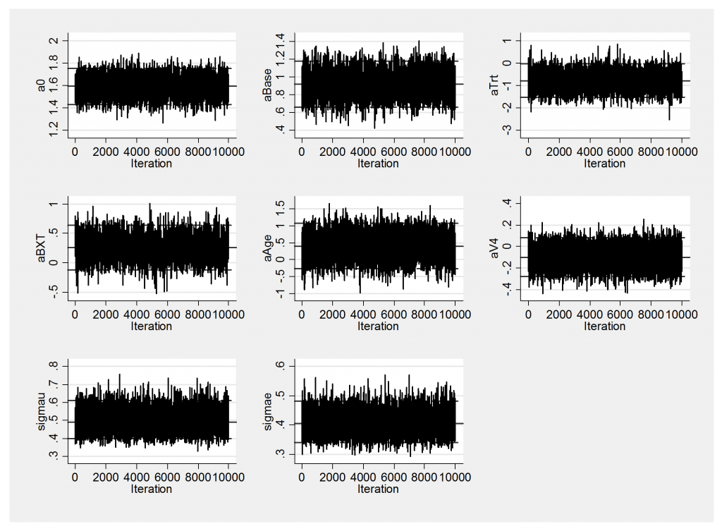
Notice how the sem for aBase has reduced from 0.0048 to 0.0029 and for aTrt has reduced from 0.0193 to 0.0068. Very roughly we have halved the standard errors on the three highly correlated parameters aBase, aTrt and their interaction aBXT suggesting that WinBUGS would need to be run for roughly 4 times the length of chain to obtain results equivalent to those obtained from OpenBUGS. This gain is specific to this particular problem but does fit with my overall impression that OpenBUGS is at least as good as WinBUGS and sometimes much better.
The improved mixing is also evident in the trace plot.
JAGS
Just prior to Christmas I had several postings discussing the use of JAGS with Stata (you can link to the first of those postings here). This problem gives us an opportunity to compare JAGS with the more commonly used WinBUGS and OpenBUGS. To call JAGS we need to take the Stata program given previously for calling WinBUGS and insert the jags opinion in the same places that we placed the openbugs option when we wanted to call that program. The other important change is to the wbslist calls because JAGS likes its data in a slightly different format.
I do not want to alter programs such as wbslist and wbsrun that were released at the time when Bayesian analysis for Stata was published, so I have created programs called wbslist_v2.ado, wbsscipt_v2.ado, wbsrun_v2.ado and wbscoda_v2.ado that incorporate the code needed for calling JAGS. These programs are undergoing gradual development but once they are completed and have been more thoroughly tested, I will release them as new versions of wbslist etc. In the meantime you can download the latest versions from my homepage.
wbslist_v2 knows about the special requirements of JAGS so if you specify the jags option most of the changes are made automatically for you. Where you do need to take care is when you request that text is copied directly to the data or initial values file. You do this whenever you omit the keyword that starts a bracket. In our Stata code for calling WinBUGS we specify the initial values with,
wbslist (a0=2.6, aBase=0, aTrt=0, aBXT=0, aAge=0, aV4=0, tauu=1, taue=1) ///
using init.txt , replace
The bracket does not start with a keyword such as variable or matrix and so the text is copied directly to the file.
In JAGS the data file must use <- in place of equals and each item must start on a new line without a comma. So I have introduced the _n notation to force a new line. So for JAGS we must change the Stata command to,
wbslist_v2 (a0=2.6 _n aBase=0 _n aTrt=0 _n aBXT=0 _n aAge=0 _n ///
aV4=0 _n tauu=1 _n taue=1) using init.txt , replace jags
Similarly in the creation of the data file we need to change
wbslist (var cLB cTrt cBXT clnAge) (V4=c(0,0,0,1)) ///
(struct y_1 y_2 y_3 y_4, name(y)) using data.txt , replace
to
wbslist_v2 (var cLB cTrt cBXT clnAge) (V4<-c(0,0,0,1)) ///
(struct y_1 y_2 y_3 y_4, name(y)) using data.txt , replace jags
With these changes JAGS runs as expected and takes about 1 minute 45 seconds to produce
----------------------------------------------------------------------------
Parameter         n     mean       sd     sem   median         95% CrI
----------------------------------------------------------------------------
 a0           10000    1.596    0.083   0.0023    1.597 (   1.430,   1.758 )
 aBase        10000    0.892    0.130   0.0057    0.895 (   0.635,   1.140 )
 aTrt         10000   -0.856    0.388   0.0251   -0.856 (  -1.630,  -0.132 )
 aBXT         10000    0.305    0.196   0.0179    0.307 (  -0.074,   0.693 )
 aAge         10000    0.393    0.343   0.0084    0.398 (  -0.300,   1.049 )
 aV4          10000   -0.100    0.091   0.0013   -0.100 (  -0.285,   0.080 )
 sigmau       10000    0.496    0.055   0.0006    0.492 (   0.398,   0.613 )
 sigmae       10000    0.406    0.036   0.0005    0.405 (   0.342,   0.482 )
----------------------------------------------------------------------------
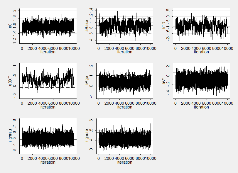
Notice how the sems on the three highly correlated parameters aBase, aTrt and their interaction aBXT are now worse than for either WinBUGS or OpenBUGS in fact they are very similar to those obtained by our program that used Stata without calling another program to do the computation. The poorer mixing is again evident in the trace plot.
Conclusions
We have to be careful about drawing conclusions from a single example but at least we have demonstrated that WinBUGS, OpenBUGS and JAGS do sometimes vary in terms of speed and mixing. We found that for this model, OpenBUGS is clearly better than WinBUGS and WinBUGS is better than JAGS. But is this fair? I have used the three programs in what we might call their default mode, that is I have not tried setting options in WinBUGS, OpenBUGS or JAGS that could have improved performance. In particular JAGS is modularized and the user can ask JAGS to add extra modules to the base release. One such module is called glm and is specifically designed to improve the performance of JAGS with this type of model.
Next time I will investigate the use of options in WinBUGS, OpenBUGS and JAGS to see if they do indeed improve performance.
Then my final challenge will be to write a Mata program that can rival these programs for speed and mixing.
The programs referred to in this posting can be downloaded from my homepage https://www2.le.ac.uk/Members/trj


 Subscribe to John's posts
Recent Comments