
Last time I analysed the epilesy data taken from Thall and Vail(1990). The model involved a Poisson regression with two random effects and I showed how this can be programmed in Stata by storing the values of the random effects in Stata variables rather than in a Stata matrix. However, the resulting do file was not very efficient and on my desktop computer it took a rather unrealistic 42 minutes to create 55,000 updates. What is worse, the mixing was quite poor so even more updates would have been necessary to produce reliable estimates.
This week I want to address the two issues of speed and mixing, although to understand the changes you will first need to read last week’s posting.
Improving the speed
First let us make the program more efficient. The do file is slow to run because I used the program logdensity to evaluate the log-densities of the distributions that make up the posterior. Use of logdensity simplifies the coding but it evaluates terms in the densities that are constant and which could have been dropped from the calculation without altering the posterior. What is more, logdensity repeatedly checks the inputs and so carries a lot overheads that slow down the program.
In our model we have a Poisson distribution in the likelihood, normal distributions over the random effects and normal and gamma priors. These distributions are simple to program so we ought to be able to speed up the calculations. In models with a few parameters, I’ve found that programming the densities directly can halve the run time over programs that use logdensity; in this model there are 303 parameters so the saving ought to be even more dramatic.
Below is a re-written version of the logpost program for the epilepsy model that does not call logdensity. It should be compared with the version that we used last week.
program logpost
args logp b
local cons = `b'[1,1]
local base = `b'[1,2]
local trt = `b'[1,3]
local bxt = `b'[1,4]
local age = `b'[1,5]
local v4 = `b'[1,6]
local tU = `b'[1,7]
local tE = `b'[1,8]
scalar `logp’ = 0
tempvar eta mu1 mu2 mu3 mu4 LL v
* log-likelihood of y_1 to y_4
gen `eta’ = `cons’ + `base’*cLB + `trt’*cTrt + `bxt’*cBXT + `age’*clnAge
gen `mu1′ = exp(`eta’ + U + E1)
gen `mu2′ = exp(`eta’ + U + E2)
gen `mu3′ = exp(`eta’ + U + E3)
gen `mu4′ = exp(`eta’ + `v4′ + U + E4)
gen `v’ = -`mu1′ + y_1*log(`mu1′) -`mu2′ + y_2*log(`mu2′) + ///
-`mu3′ + y_3*log(`mu3′) -`mu4′ + y_4*log(`mu4′)
qui su `v’ , meanonly
scalar `logp’ = `logp’ + r(sum)
* log-density of the random effects
qui replace `v’ = -0.5*`tE’*(E1*E1 + E1*E2 + E3*E3 + E4*E4) – 0.5*`tU’*U*U ///
+ 2*log(`tE’) + 0.5*log(`tU’)
qui su `v’ , meanonly
scalar `logp’ = `logp’ + r(sum)
* priors
scalar `logp’ = `logp’ -0.5*(`cons’-2.6)^2 -0.5*(`base’-1)^2 + ///
-0.5*`trt’*`trt’ -0.5*`bxt’*`bxt’ -0.5*`age’*`age’ -0.5*`v4’*`v4′ + ///
7*log(`tU’) – 2*`tU’ + 7*log(`tE’) – 2*`tE’
end
The improvement is speed is dramatic. The original version took 42 minutes to produce 55,000 iterations of the sampler, while this new version takes 6 minutes, faster by a factor of 7.
Improving the mixing
Unfortunately the improvement in speed does nothing for the mixing which is still very poor as this trace plot shows.
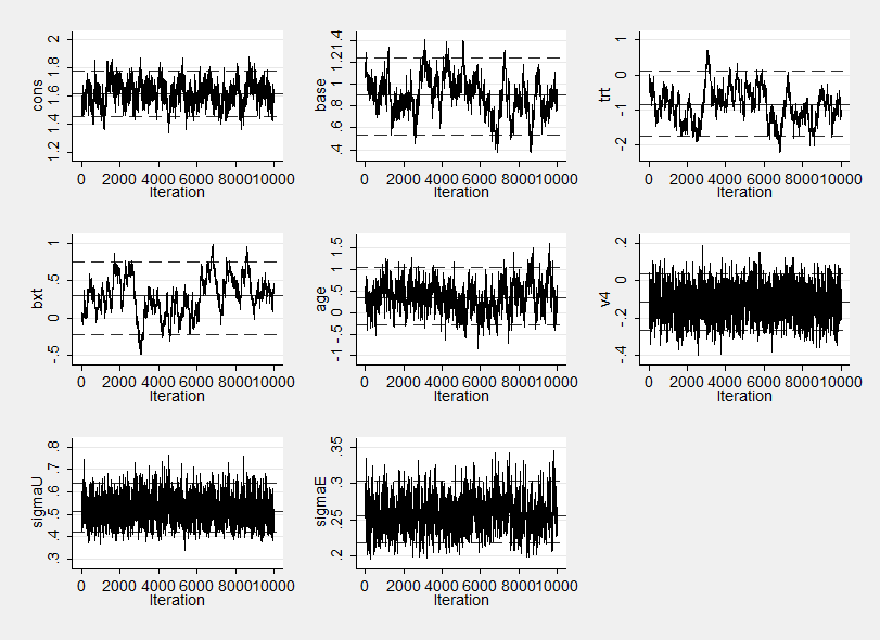
I ran mcmcstats to obtain summary statistics from the saved results and added the correlation option in order to help me diagnose the cause of the problem. Not surprisingly the three parameters that mix poorly, namely base, trt and bxt (basextrt interaction) are all highly correlated.
        |    cons base     trt     bxt     age    v4 sigmaU sigmaE
 -------+----------------------------------------------------------
 cons   | 1.0000
 base   | -0.1506 1.0000
 trt    | -0.0661 0.7239 1.0000
 bxt    | 0.0521 -0.7922 -0.9514 1.0000
 age    | -0.0020 -0.0817 -0.1465 0.2038 1.0000
 v4     | -0.2659 0.0258 0.0388 -0.0382 -0.0493 1.0000
 sigmaU | -0.0796 0.0131 0.0387 -0.0543 -0.0155 0.0398 1.0000
 sigmaE | -0.0495 -0.0639 -0.0678 0.0783 -0.0732 0.0744 -0.0104 1.0000
One tactic for handling correlated parameters is to use a multivariate normal proposal so that the three parameters are updated in a single step, then we can choose the new multivariate proposal to allow for the anticipated correlation.
The multivariate normal proposal version of the Metropolis-Hasting algorithm described in the book is called mhsmnorm and this takes the Cholesky decomposition of the variance matrix as its input. We do not need an exact value for this matrix so it is not important to base it on exact correlations or standard deviations. The proposal distributions for the three troublesome parameters as produced by the current algorithm are 0,17, 0.49 and 0.26 so we can obtain the Cholesky decomposition by,
matrix R = (1, 0.70, -0.80 \ 0.70, 1, -0.95 \ -0.80, -0.95, 1)
matrix sd = (0.17, 0.49, 0.26)
matrix D = diag(sd)
matrix C = D*R*D
matrix L = cholesky(C)
matrix list L
and we obtain
c1 c2 c3
c1 .17 0 0
c2 .343 .34992999 0
c3 -.208 -.1419884 .06461652
The only change that we need to make is to replace the three normal proposal calls to mhsnorm for base, trt and bxt with a single call to mhsmnorm with L set close to this Cholesky matrix.
matrix L = (0.17, 0, 0 \ 0.343, 0.350, 0 \ -0.208, -0.142, 0.065)
mhsnorm `logpost’ `b’ 1, sd(0.1)
mhsmnorm `logpost’ `b’ 2, chol(L)
mhsnorm `logpost’ `b’ 5, sd(0.1)
In fact these steps are a little large and trial and error shows that we get slightly better performance with L/4 that is with shorter steps with the same correlation.
The trace plot is now
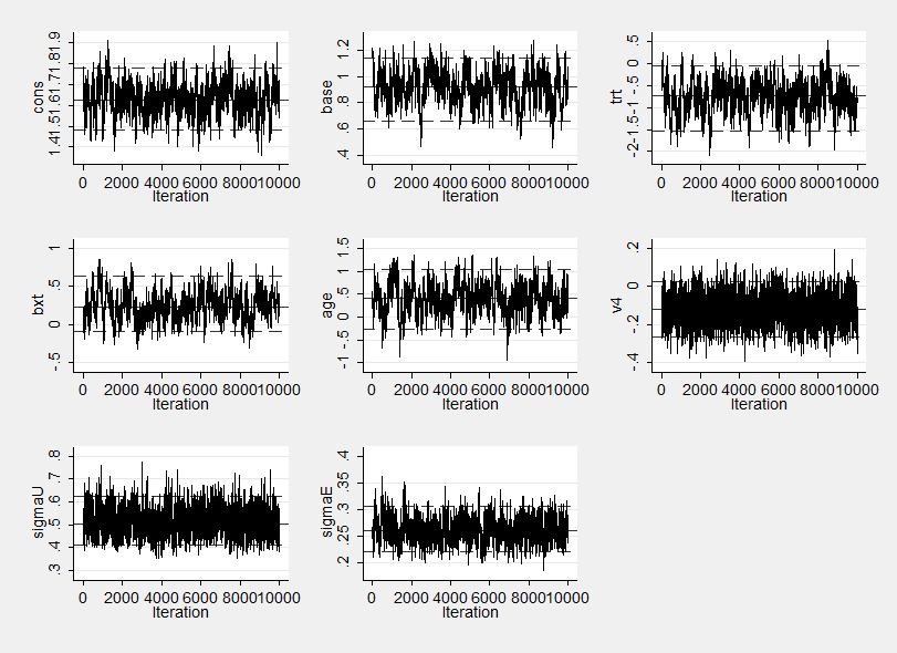
The new summary statistics are,
----------------------------------------------------------------------------
Parameter         n     mean       sd      sem   median         95% CrI
----------------------------------------------------------------------------
 cons         10000    1.593    0.081   0.0039    1.593 (   1.432,   1.746 )
 base         10000    0.904    0.125   0.0078    0.905 (   0.667,   1.146 )
 trt          10000   -0.764    0.368   0.0212   -0.780 (  -1.477,  -0.004 )
 bxt          10000    0.254    0.181   0.0109    0.256 (  -0.105,   0.599 )
 age          10000    0.408    0.307   0.0147    0.414 (  -0.199,   0.993 )
 v4           10000   -0.099    0.090   0.0022   -0.099 (  -0.271,   0.077 )
 sigmaU       10000    0.492    0.053   0.0009    0.488 (   0.398,   0.606 )
 sigmaE       10000    0.409    0.037   0.0011    0.409 (   0.339,   0.481 )
----------------------------------------------------------------------------
Tuning the proposal standard deviations
Another way to improve the mixing is to use better standard deviations for the proposal distributions. The program mcmcrun has an adapt option, which when set instructs the program to adapt the proposal standard devaitions during the burn-in phase by increasing them when a proposal is accepted and decreasing them when a proposal is rejected. As we are using our own sampler we cannot use this automatic facility but we can program it for ourselves.
First I declared a global called NITER that started at zero and was updated by one in our sampler every time was called. The starting values of the proposal standard deviations were stored in a row matrix called SD. Then, depending on the current value of NITER, the program would call the sampler mhsEPY or a new version called mhsEPYburnin. mhsEPY works just as before but mhsEPYburnin modifies the contents of SD depending on whether a proposal is accepted as not.
I will not list the code but it can be downloaded with the other programs from my homepage. Using this adpatation the results were,
----------------------------------------------------------------------------
Parameter         n     mean       sd      sem   median         95% CrI
----------------------------------------------------------------------------
 cons         10000    1.597    0.080   0.0033    1.596 (   1.446,   1.757 )
 base         10000    0.930    0.129   0.0087    0.928 (   0.675,   1.181 )
 trt          10000   -0.776    0.362   0.0225   -0.770 (  -1.500,  -0.074 )
 bxt          10000    0.267    0.187   0.0124    0.269 (  -0.098,   0.637 )
 age          10000    0.419    0.334   0.0136    0.429 (  -0.261,   1.054 )
 v4           10000   -0.102    0.092   0.0021   -0.102 (  -0.280,   0.083 )
 sigmaU       10000    0.495    0.055   0.0009    0.491 (   0.397,   0.611 )
 sigmaE       10000    0.409    0.035   0.0008    0.407 (   0.344,   0.481 )
----------------------------------------------------------------------------
In fact the sem do not change much because my original guesses for the proposal standard devaitions were reasonable.
If we compare these with the results that were obtained last week we see that for the same number of iterations the sem’s have reduced dramatically. For base 0.0145 has become 0.0087, for trt 0.0526 has become 0.0225, for the interaction 0.0417 has become 0.0124.
These improvements roughly halve the sem which means that to obtain our new performance the old program would need to have been run for 4×55000 =220,000 iterations and even with the new efficient coding of logpost this would take 24 minutes rather than the current 6 minutes.
Combined effect
The modifications that we have made have not changed the answer but they do make a dramatic difference to the performance. We have reduced the run time by a factor of 7 by recoding logpost and by a factor of 4 by improving the mixing. A combined factor of 28 so that something that previously took 1 minute now takes about 2 seconds.
No doubt the code could be made even quicker and the mixing could be improved even further but additional changes are unlikely to have such a marked impact and would probably not justify the effort. If we want further improvements then we need to switch to Mata or WinBUGS and I’ll consider that possibility next time.
Meanwhile the programs referred to in this posting can be downloaded from my homepage https://www2.le.ac.uk/Members/trj

 Subscribe to John's posts
Recent Comments