In my last posting I introduced a program for comparing different methods of convergence assessment in multi-dimensional MCMC analyses. Essentially the program samples from an imaginary posterior that takes the form of a user specified mixture of multivariate normal distributions. Previously, I illustrated some of the problems of assessing convergence by looking at a simulated chain from a single three dimensional normal distribution. This time I would like to assess convergence when the posterior takes the form of a mixture of two normal distributions.
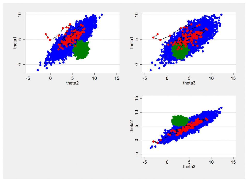
To start with, I simulated an artificial chain from a mixture of a wide-ranging normal distribution which represents 80% of the posterior and a much tighter normal distribution that represents the other 20%. The chain had high autocorrelation (0.95) so I chose to simulate 100,000 updates and then thinned by 5 to leave 20,000. Here is a plot of the chain with the first 100 points shown in red and the two components of the mixture shown in blue and green. Remember that although the simulation is created from two separate components the posterior is a single bimodal distribution.
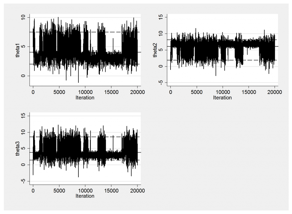
The chain finds both components but spends about 35% of its time in the smaller component rather than the desired 20%, so the posterior is not well represented. Because of the high autocorrelation the chain tends to stay in whichever part of the posterior that it finds itself. We can see this clearly from the trace plot that shows the poor mixing between regions. Once in the tighter mode the chain tends not to move to the outer regions of lower probability and once outside the other mode the chain can move far enough away that it does not find the first mode again for a while.
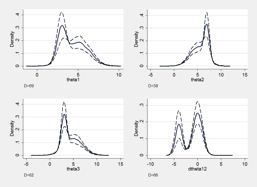
The section plots better demonstrate that the proportions of the chain in the two regions have not yet converged. I deliberately placed the second component so that its mode is slightly offset in the direction of theta1-theta2 and so I have included the section plot for the derived parameter dtheta12=theta1-theta2. In this plot the bimodel nature of the distribution is more evident and illustrates how, in multi-dimensional models, we can miss important features if we only look at simple marginal posterior distributions.
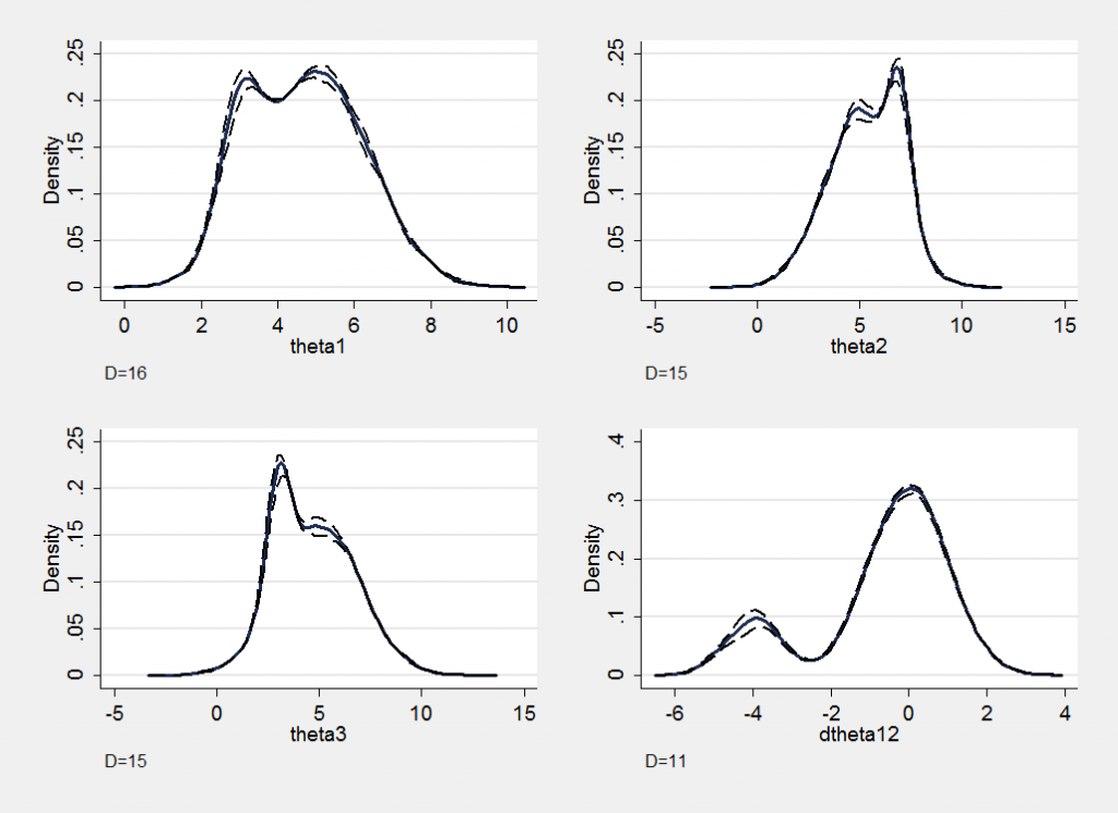
Here are the section plots for a new chain identical in every respect to the first except that it is produced with an autocorrelation of 0.50 instead of 0.95. The lower autocorrelation makes it more likely that the algorithm will switch between the main mode and the rest of the posterior and the new chain represents this particular non-normal posterior reasonably accurately. If we were unable to design a sampler with a lower autocorrelation we would have had to adopt the brute force solution of running a much longer chain.
The trace plots alert you to poor mixing but will give no indication whether the chain has been run for long enough; section plots are much more useful although even these can be misleading if important features lie in directions that do not correspond to the current parameterization.
Perhaps the hardest problems arise in models with scores or even hundreds of parameters of which just a few exhibit this type of bimodal shape in the posterior. It is very demanding to insist that the marginal plots of every parameter are inspected to pick up the few that have a problem. As Bayesian models get more complex there is a serious need for programs that automatically search through the MCMC results and only print out the plots for those parameters that have a possible problem. For instance it would be easy to write a program that calculates the D statistic for each of 100 parameters but which only plots the section plots for, say, the worst 10 or those with D below some specified level. Such a search becomes even more demanding if want to ensure that there are no important features hidden from us by the current choice of parameterization.
This will be my last posting for a few weeks as I will be working abroad. I will post again in the second half of July.


 Subscribe to John's posts
Hi there friends, nice paragraph and nice arguments commented at this place,
I am genuinely enjoying by these.
First of all I would like to say fantastic blog!
I had a quick question that I’d like to ask if you don’t mind.
I was interested to know how you center yourself and clear
your thoughts prior to writing. I have had a tough time clearing my thoughts in getting
my thoughts out there. I do take pleasure in writing but it just seems like the first 10 to
15 minutes are usually lost just trying to figure out how to begin. Any recommendations or tips?
Appreciate it!
I pleased that you enjoy the blog.
Writing does not come naturally to me, so I have been forced to develop an approach that works for me. I always try to have a clear structure in my mind before I start. Most of my postings are written around a particular piece of Stata code, so that example creates its own structure. One advantage that I do have, is that I have been teaching statistics for many years and I have learnt to appreciate the types of ideas that people find difficult and those which are are easily misunderstood. In my experience, people are capable of understanding very complex ideas if they are explained in a non-technical way. When students are confused about something, it is often because the teacher does not really understand it themselves. So here are my tips (a) decide on the structure before you start (b) write simply and avoid technical terms (c) create a first draft quite quickly and then make lots of edits to improve the clarity.
I am extremely impressed along with your writing skills as well as with the format
to your blog. Is that this a paid subject matter
or did you customize it yourself? Either way stay up the
nice quality writing, it’s uncommon to see a great blog like this one these days..
I am pleased that you find the blog helpful – I write it purely as a hobby because the subject interests me, although of course the topics that I cover overlap with the book that I wrote and with some of my teaching. As to writing skills, when I was at school I was always near the top of the class in mathematics and near the bottom of the class in English. My old English teachers would be pleasantly surprised by your comment. I still find writing quite hard.
It’s really a nice and helpful piece of information. I am glad
that you just shared this helpful info with us. Please stay us up to date like this.
Thanks for sharing.
thank you for your kind remarks – feedback like this is helpful in encouraging me to keep going
Generally I do not learn article on blogs, but I would like to say that this write-up very compelled me to check
out and do it! Your writing taste has been surprised me.
Thank you, quite great article.
thank you for those kind words
Hi! Very interesting post.
I wonder: with a bimodal posterior and a high autocorrelation, other than running the chain for very long as you say (and I guess with a high thinning interval??), would it help to run it in Stan compared to JAGS?? Would Hamiltonian MCMC as implemented in Stan help explore the posterior distribution more effectively, so that fewer iterations are required??
My experience is that Stan is very good in situations when there is strong correlation between parameters but I rather doubt its algorithm would offer a solution the bimodal problem. HMC performs loops around contours of the posterior but in the bimodal case the contours would consist of two separate sets of rings and I suspect that you would tend to stay within the set that you started in. However, I’ve not tried it for myself so it is worth investigating.
Ziemlich verrückter Beitrag, den Sie da gepostet haben. Wussten Sie schon eine gute Lösung für die Problemstellung?
Nein, ich diskutiere nur, was in meinem kopf zu der zeit ist
Ganz erstaunlicher Beitrag, was Sie da gepostet haben. Wissen Sie bereits eine vernünftige Lösung für das Problem?
Dies ist ein vernachlässigtes Thema, das viel mehr Forschung braucht
I agree, john