Stan with Stata, Part V: Kicking a marble around in a bucket

In the last few postings I have described how the Bayesian analysis program, Stan, can be called from within Stata. Before we can go any further we have to understand how Stan works, which is to say we need to understand the basics of Hamiltonian Monte Carlo, as this is Stan’s way of sampling from the posterior.

I’ll start the explanation this week and complete it next time.

The problem with Gibbs Sampling
WinBUGS, OpenBUGS and JAGS are all based on Gibbs Sampling, hence the GS in each of their names. Gibbs samplers work by moving through the set of parameters in some defined order, updating one set of parameters, then moving on to update the next. Each time the sampling is controlled by the conditional distribution of the current set of parameters fixing all others at their current values.

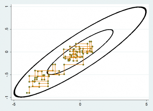
Gibbs samplers reduce multi-dimensional problems to a long sequence of low dimensional moves and as such are simple to program. Their chief disadvantage is illustrated in the diagram below. Here we have two parameters with a reasonably high correlation and we update them one at a time holding the other parameter at its current value. The result is that we tend to make very local moves and it can take a long time to get from one end of the distribution to the other. Hence poor mixing and an inefficient algorithm.

Ideally we would like a sampler that takes the multi-dimensional shape of the posterior into account and that is able to move more quickly across the distribution. Block updating, in which correlated parameters are grouped together in the Gibbs sampler is an attempt to do this, but it requires that the user understand the shape of the distribution when they are designing the sampler and so it is not truly automatic.

Hamiltonian Monte Carlo

Hamiltonian Monte Carlo (HMC) is an alternative to Gibbs sampling that is designed to give better mixing when parameters are correlated, but without the user needing to have advance knowledge about the shape of the posterior. Sometimes HMC is called Hybrid Monte Carlo.

Many years ago, I studied mathematics at University and in my first year they made us study pure maths, applied maths and statistics. As much as anything else, it was my inability to do applied maths that made me become a statistician. The equations of motion of a spinning top were a mystery to me but I remember that at the end of the year we reached the Lagrangian and the Hamiltonian. Unfortunately, by that stage, I had lost what little intuition I had for mechanics.

If you understand Hamiltonian mechanics then the parallels will help you to understand HMC and you will probably love the chapter by Radford Neal called MCMC using Hamiltonian Dynamics in the Handbook of Markov chain Monte Carlo published by Chapman and Hall. If, on the other hand, you are like me, then you will need a gentler approach.

It is actually quite difficult to talk about HMC without using physical analogies but let’s try to avoid diving into Hamilton’s equations of motion. Instead let’s start by imagining a much simpler algorithm for a one dimensional parameter, θ, with posterior f(θ). We start with a random guess θ_t and then update iteratively such that,
θ_t+1 = θ_t + ε df/dθ
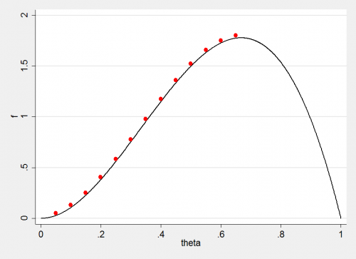
where the derivative is evaluated at the current point. This is a crude hill climbing algorithm that makes steps of size ε with the direction and magnitude of the gradient. When we reach the top of the hill the gradient will be zero and we will stay there. What we have is an algorithm for finding the mode of the posterior.

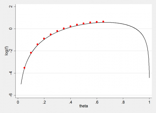
Of couse we could equally well work on the log-scale and the value of θ at the mode would not change.

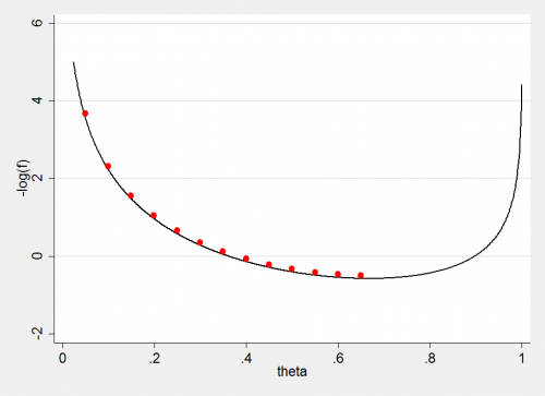
Alternatively we could invert the curve and use the method to find the minimum rather than the mode.

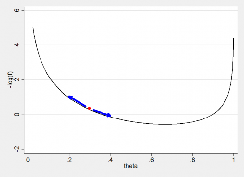
With a hill climbing or descending  algorithm, we naturally think of it as making a series of discrete steps, but we could make the step length very small and imagine a continuous path from our initial guess to the mode. We would find that the speed of movement is greater when we pass through a steep region of the hill. My analogy is with a marble rolling inside a bucket.

Now this is an aspect of the algorithm does does not come across in these two dimensional pictures; the bucket is multi-dimensional because in this algorithm all of the parameters are handled simultaneously. So the shape of the bucket reflects all of the correlations within the parameters and the algorithm automatically adjusts whatever the multi-dimensional shape of the posterior.

One other point to notice is that this journey is entirely deterministic, the movement depends only on the current position and the slope at the current position, it does not depend on the route that we took to get there and so we could reverse the algorithm and deduce the path that we must have taken.

If you believe in maximum likelihood estimation, then make f the likelihood and this algorithm would find the MLE. It has its problems; for instance, we have to be careful when choosing the step length and starting value or the algorithm might settle on a local mode when there is a higher mode somewhere else.

But we are Bayesians, so our hill represents a posterior distribution and we want to characterise its whole shape so that we will be able to find the mean of θ rather than the mode. So we do not want to settle at the mode but instead we need to keep travelling over the distribution.

To keep the movement going, we allow the marble to move deterministically within the multi-dimensional bucket but periodically we give it a random kick. We might decide to allow the parameter to move for a fixed time or for, say, 10 discrete steps then kick it again and let it move for another ten steps and so.

We want to do this in such a way that the values of the parameter at the end of each set of 10 small steps act like a random sample from the posterior. The key is how the marble moves after we give it a kick. This problem has already been solved by the equations of motion of mechanics and a neat formulation of those equations was provided by the Irish mathematician, Hamilton, who used the conservation of energy to describe the motion. In our analogy the shape of the surface provides the marble with potential energy and the kick imparts kinetic energy. Balancing changes in one against changes in the other allows us to deduce the path.

In turns out that if the kick has a size (momentum) z, we can update
θ_t+1 = θ_t + e z_t
and then the energy in the kick is lost in such a way that,
z_t+1 = z_t – e df/dθ
where f is  minus the log-posterior (shape of the surface which dictates the potential energy). These two equations are a special case in which the momentum of the kick is drawn independent of position from a distribution g such that
d/dz[ -log(g) ] = z
which amounts to g = exp(-z²/2) which of course is proportional to a N(0,1) distribution. This is a very convenient way to generate the random kicks, but it is not the only way.

Let us see how this works in practice. Suppose that the posterior is a beta distribution, B(3,2) so
it is proportional to θ²(1-θ)
f = -2logθ – log(1-θ)
df/dθ = -2/θ+1/(1-θ)
There are a lot of tuning parameters in this algorithm, but for my example I will choose to make sets of 20 steps of size 0.01. In all, I will generate 500 values from the posterior.
clear
* 500 sets of 20 steps
set obs 500
gen theta = 0
gen z = 0
local eps = 0.01
* random starting value
local t = runiform()

forvalues iter=1/500 {
* a random kick
    local z = rnormal()
* twenty steps
    forvalues i=1/20 {
       local z = `z’ – `eps’*(-2/`t’+1/(1-`t’))
       local t = `t’ +`eps’*`z’
    }
    qui replace theta = `t’ in `iter’
    qui replace z = `z’ in `iter’
}
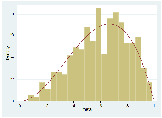
histogram theta , addplot(function y = 12*x*x*(1-x) , range(0 1)) leg(off)

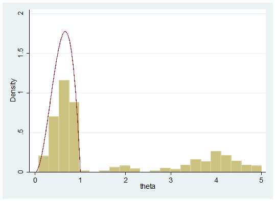
Amazingly successful for such a simple piece of code, but it can go wrong. Here is another random sample generated by the same code,

Of course this should not happen because theta ought to stay between 0 and 1, but if, due to the finite size of the step, we do veer outside this range then the algorithm can go wild. Think of the analogy with badly tuned mode finding algorithms that diverge away from the peak, or of someone kicking the marble out of the bucket.

Enough for one week. More on HMC next time.