Stan with Stata, Part VI: More about HMC

Last time I discussed the HMC (Hamiltonian Monte Carlo or Hybrid Monte Carlo) algorithm that forms the basis of Stan and I likened the algorithm to kicking a marble around in a bucket. The multi-dimensional shape of the bucket is defined by minus the log-posterior and the marble represents the current value of the estimator. We give the marble a random kick and monitor its path, after a fixed time we note the position and give it a random kick in a new direction. The set of all of the positions at the times of the kicks represents the sample from the posterior.

One of the big advantages of HMC is that it updates all of the parameters together and because it uses the multi-dimensional shape of the log-posterior, it automatically allows for the correlations between the parameters.

In the previous posting, we looked at a simple example based on a beta distribution and found that HMC is numerically sensitive to a number of tuning parameters. Stan’s real achievement is not that it has programmed HMC, we did that ourselves in a dozen lines of Stata code, but rather that Stan has found ways to tune the algorithm and to make it efficient and numerically robust.

The example of the univariate beta distribution hid one of the main practical difficulties with HMC, which is that we need the derivatives of the log-posterior in order to define the path of the estimator. This was not an issue for the one dimensional example but it is a serious concern for a multi-dimensional model. Stan comes to the rescue once again by building accurate differentiation into the program.

Because Stan has automated the algorithm in a very intelligent way, you could treat it like a black box and trust to the defaults and if you do so, you will often get very good results. However, with more complex models you might need to alter the algorithm by, for example, setting a different step length. All of the (many) tuning decisions can be controlled using command line options when you call Stan, but to set them intelligently requires a deeper understanding, not so much of the HMC algorithm, as of its numerical implementation.

This week I will give a few more details so that you can understand when you read the manual and see reference to leapfrogging and NUTS, but I will not try to be comprehensive. I think that it is better to gain some experience of using the algorithm before we try to understand its deeper secrets.

Let us start with the basic algorithm, which represents the continuous path of the marble in the bucket by a set of discrete steps of length ε,
z_t+1 = z_t – ε df/dθ
θ_t+1 = θ_t + ε z_t
where θ is the estimate, f is the log posterior and z is the momentum which is periodically given a random kick drawn from a multivariate normal density. For the one dimensional beta model, I implemented this as by the Stata code,
local z = `z’ – `eps’*(-2/`t’+1/(1-`t’))
local t = `t’ +`eps’*`z’
where the local t contained the current value of theta.

If we think of the steps of size ε as being used to approximate a continuous path, then instead of updating z by ε and then t by ε, we could update z by ε/2 then update t by ε then update z by the other ε/2.
local z = `z’ – 0.5*`eps’*(-2/`t’+1/(1-`t’))
local t = `t’ +`eps’*`z’
local z = `z’ – 0.5*`eps’*(-2/`t’+1/(1-`t’))
This is called leapfrogging and gives changes that are closer to the continuous path.

We can think of the total effect of the set of steps as a transformation that maps one pair (t,z) into a new pair (t’,z’) and as such the transformation will have a Jacobian. One important property of the leapfrog is that it always has a Jacobian of one, so that we never need to calculate it.

Since we are using zigzagging discrete steps to approximate a continuous path it would be surprising is some small numerical error did not creep in after we have made a complete set of steps. So our calculated (t’,z’) will not be exactly on the continuous path. To adjust for this inaccuracy, Stan introduces a Metropolis step to decide whether to accept the calculated pair from the end of the set of moves or to stay with the previously selected pair. The Metropolis accept/reject test is such that, were we exactly on the continuous path, then the acceptance probability would be one.

So we have a complex trade off; we want small steps in order to stay close to the continuous path, but small steps mean that we do not move very far, so the chain will show high autocorrelation. Increase the step length or take more steps and we will move further, but we are more likely to deviate from the correct path, then the new point might be rejected in the Metropolis step and once again we will have high autocorrelation.

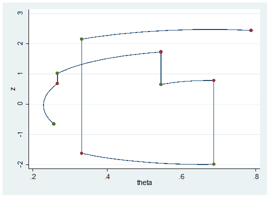
To understand the impact of the number of steps let us use the Stata code that we had last week but instead of simulating many sets of steps we will only take a few sets but we will plot the whole path rather than just the end point.

clear
set obs 100
gen theta = 0
gen z = 0
local eps = 0.01
* random starting value
local t = runiform()
local k = 0
forvalues iter=1/5 {
* a random kick
local z = rnormal()
local ++k
qui replace theta = `t’ in `k’
qui replace z = `z’ in `k’
* twenty steps
forvalues i=1/20 {
local z = `z’ – `eps’*(-2/`t’+1/(1-`t’))
local t = `t’ +`eps’*`z’
local ++k
qui replace theta = `t’ in `k’
qui replace z = `z’ in `k’
}
}
twoway (line z theta) (scatter z theta if mod(_n,20) == 0 ) ///
(scatter z theta if mod(_n,20) == 1 ), leg(off)

In the plot a green dots represent the start of a set of 20 steps and a red dot represent the end of a set and therefore the new simulated value of theta. The vertical jumps are the random kicks given to z.

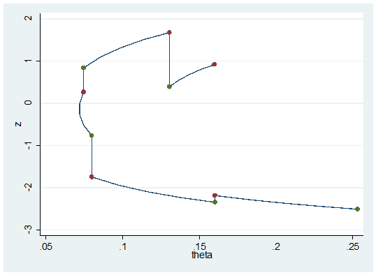
What happens if we run for two few iterations or use too small a step length. Below I keep the same step length but only make 5 steps instead of 20.

Notice the scale of theta! We do not move very far, the pairs of green and red dots have similar values of theta and so the chain will show high autocorrelation.

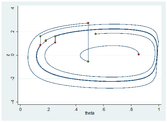
Now we will change to 100 steps of length 0.01.

The path tends to complete a cycle and if we are unlucky we will end very close to the place where we started and again we will have high autocorrelation in the chain. Even if we do move, going round and round the same path is a very inefficient way to progress.

To improve the tuning of the HMC, Stan uses the no U-turn algorithm (NUTS). Essentially this means monitoring the distance from the starting point and stopping when we first turn back on ourselves. There is a slight problem with this in that it is not reversible. Imagine moving clockwise around a long thin ellipse by starting half way along the upper long side. You would stop close to the right-hand end as you turn the corner. Now work anti-clockwise from your finishing point. You would go all of the way to the left hand end of the ellipse before stopping. The fact that the paths are not reversible alters the target distribution and so we will not get the posterior that we were hoping for. NUTS corrects for this by running two paths, one forwards and one backwards and then sampling from those paths in such a way that the moves are probabilistic, but with probabilities that are reversible.

I understand that I have left many gaps in this description of HMC and any mathematician reading this would probably be reduced to tears, but I honestly believe that this level of understanding is sufficient to enable you to use Stan and, hopefully, some people will be stimulated to want to read the mathematics behind the algorithm.

Here are some references for those who want the details.

Homan, Matthew D., and Andrew Gelman. “The no-U-turn sampler: Adaptively setting path lengths in Hamiltonian Monte Carlo.” The Journal of Machine Learning Research 15.1 (2014): 1593-1623.

Neal, Radford M. “MCMC using Hamiltonian dynamics.” in Brooks, Steve, et al., eds. Handbook of Markov Chain Monte Carlo. CRC press, 2011.

Chen, Lingyu, Zhaohui Qin, and Jun S. Liu. “Exploring hybrid monte carlo in bayesian computation.” ISBA and Eurostat 6 (2001): 2-1

Beskos, Alexandros, et al. “Optimal tuning of the hybrid Monte Carlo algorithm.” Bernoulli 19.5A (2013): 1501-1534.

Next time I will take a more realistic example and run a competition, Stan vs WinBUGS.