
Most of my postings are based on bits of code that were produced for other reasons; perhaps for my teaching or for my research or sometimes they are left over from when I was writing the book on Bayesian Analysis with Stata. So typically I spend a couple of hours each week on the blog; an hour for playing with the code and an hour for writing the text. This week’s posting took me over five hours! I made a silly mistake in the code and I simply could not spot it.
I described the data augmentation algorithm in a posting just before Easter. It uses the fact that when events occur at random with a constant rate, the number of events in a fixed time follows a Poisson distribution and the intervals between the events follow an exponential distribution. So one way to analyse a Poisson regression model is to simulate the times between events and then to analyse those with an exponential model. Easy to code, so even though I had not written a program for this algorithm before, I was not anticipating any problems.
I took the Poisson counts from the epilepsy trial that has occupied this blog since February, I simulated the random event times and I analysed them with a Gibbs sampler based on an exponential model. Of course, it did not work.
The Gibbs sampler for this problem is slightly unusual because the signs are different to those that you usually associate with a linear predictor. The mean of the exponential is one over the mean of the Poisson, so on a log-scale we get an extra minus sign when we switch from the Poisson to the exponential. I became obsessed with the signs and I checked them and checked them again and again. I even did the thing that I tell my students that they should never do. I resorted to making arbitrary changes to the signs in the hope that a miracle would happen. It rarely does.
At five O’clock on the last working day before Easter the program was still not working and I decided that enough is enough. Then, as I was about to close Stata, I saw the error. There must be something psychological going on because I have noticed before that one sees in a moment of relaxation what one misses during forced concentration. Anyway it had nothing to do with the signs, rather I had analysed the simulated times of the events instead of the simulated intervals between the events.
Since I sweated over this program, I will reproduce it in full. I explained before Easter how we can approximate the log-exponential by a mixture of five normal distributions. This reduces the problem to a normal errors regression model that can be fitted by a Gibbs sampler. I have added the derivation of the Gibbs sampler to my formula sheet which can be downloaded as a pdf from here, augmentationGS.
Here is the code
*———————————————
* Switch to Mata
*———————————————
set matastrict on
mata:
mata clear
void dummy()
{
}
void mygibbs(real scalar logp,pointer(function) logpost,real matrix X,
real rowvector theta,real scalar ip)
{
rowvector wMix, mMix, vMix, sdMix, priorMean, priorPrecision
real scalar i, j, k, kend, sumBeta, sumBetaSq, r, mu
real colvector time, u, eta, sf, y, p, ivDeviation, precision,
etaPoisson, vk, mk, xj
real matrix f
// parameters of the normal mixture
wMix = (0.2924,0.2599,0.2480,0.1525,0.0472)
mMix = (0.0982,-1.5320,-0.7433,0.8303,-3.1428)
vMix = (0.2401,1.1872,0.3782,0.1920,3.2375)
sdMix = sqrt(vMix)
// linear predictor for the Poisson log-mean
etaPoisson = theta[1]:+theta[2]:*X[,2]:+theta[3]:*X[,3]:+theta[4]:*X[,4]:+
theta[5]:*X[,5]:+theta[6]:*X[,6]:+X[,7]:+X[,8]
// Simulate the times
time = J(2184,1,0) // augmented intervals
eta = J(2184,1,0) // eta for the augmented intervals
p = J(2184,1,0) // data row corresponding to the augmented data
k = 0
for(i=1;i<236;i++ ) {
for(j=2;j<=X[i,1];j++) {
time[k+j-1] = u[j] – u[j-1]
eta[k+j-1] = etaPoisson[i]
p[k+j-1] = i
}
}
k = k + X[i,1]
time[k] = 1 – u[X[i,1]] – log(runiform(1,1))/mu
eta[k] = etaPoisson[i]
p[k] = i
}
}
// estimate the component of the mixture
f = J(2184,5,0) // densities of normal components
sf = J(2184,1,0) // sum of the densities
y = log(time) + eta // augmented observation
for(r=1;r<=5;r++) {
f[,r] = wMix[r]:*normalden(y,mMix[r],sdMix[r])
sf = sf + f[,r]
}
f[,1] = f[,1]:/sf
for(r=2;r<=4;r++) {
f[,r] = f[,r]:/sf + f[,r-1]
}
u = runiform(2184,1)
vk = J(2184,1,1) // variance of kth log(time)
mk = J(2184,1,1) // mean of kth log(time)
for(k=1;kf[k,1]) + (u[k]>f[k,2]) + (u[k]>f[k,3]) + (u[k]>f[k,4])
vk[k] = vMix[r]
mk[k] = mMix[r]
}
// Gibbs sampling
priorMean = (2.6,1,0,0,0,0)
priorPrecision = (1,1,1,1,1,1,1)
// update the regression coef
xj = J(2184,1,1)
for(j=1;j 1 ) xj = X[p,j] // the covariate corresponding to term j
y = y:-theta[j]:*xj
sumBeta = priorMean[j]*priorPrecision[j] – sum(xj:*(y-mk):/vk)
sumBetaSq = priorPrecision[j] + sum(xj:*xj:/vk)
theta[j] = rnormal(1,1,sumBeta/sumBetaSq,1/sqrt(sumBetaSq))
y = y:+theta[j]:*xj
}
// u’s
y = y – X[p,7]
ivDeviation = (y:-mk):/vk // inverse variance deviation
precision = 1:/vk // precisionsof each augmented observation
for(i=1;i<=59;i++) {
sumBeta = 0
sumBetaSq = theta[7]
for(k=1;k<=2184;k++) {
if( p[k] == i | p[k] == i+59 | p[k] == i+118 | p[k] == i+177 ) {
sumBeta = sumBeta – ivDeviation[k]
sumBetaSq = sumBetaSq + precision[k]
}
}
X[i,7] = rnormal(1,1,sumBeta/sumBetaSq,1/sqrt(sumBetaSq))
X[i+59,7] = X[i,7]
X[i+118,7] = X[i,7]
X[i+177,7] = X[i,7]
}
y = y + X[p,7]
theta[7] = rgamma(1,1,37.5,1/(2+0.5*X[|1,7\59,7|]’*X[|1,7\59,7|]))
// e
y = y – X[p,8]
ivDeviation = (y-mk):/vk
for(i=1;i<=236;i++) {
sumBeta = 0
sumBetaSq = theta[8]
for(k=1;k<=2184;k++) {
if( p[k] == i ) {
sumBeta = sumBeta – ivDeviation[k]
sumBetaSq = sumBetaSq + precision[k]
}
}
X[i,8] = rnormal(1,1,sumBeta/sumBetaSq,1/sqrt(sumBetaSq))
}
y = y + X[p,8]
theta[8] = rgamma(1,1,126,1/(2+0.5*X[,8]’*X[,8]))
}
end
*———————————————
* back to Stata
*———————————————
use epilepsy.dta , clear
gen LB = log(Base/4)
qui su LB
gen cLB = LB – r(mean)
gen lnAge = log(Age)
qui su lnAge
gen clnAge = lnAge – r(mean)
gen BXT = LB*Trt
qui su BXT
qui gen cBXT = BXT – r(mean)
qui su Trt
gen cTrt = Trt – r(mean)
gen id = _n
gen zero = 0
gen one = 1
stack id y_1 cLB clnAge cTrt cBXT zero id y_2 cLB clnAge cTrt cBXT zero ///
id y_3 cLB clnAge cTrt cBXT zero id y_4 cLB clnAge cTrt cBXT one , ///
into(id y cLB clnAge cTrt cBXT v4)
rename _stack visit
sort visit id
matrix theta = J(1,8,0)
matrix theta[1,1] = 2.6
matrix theta[1,2] = 1
matrix theta[1,7] = 4
matrix theta[1,8] = 4
gen u = rnormal(0,0.5) in 1/59
forvalues i=1/59 {
qui replace u = u[`i’] if id == `i’
}
gen e = rnormal(0,0.5)
mcmcrun dummy X theta using mataepilepsy.csv , ///
param(cons base trt bxt age v4 tauU tauE ) ///
samp( mygibbs , dim(8) ) ///
burn(5000) update(50000) thin(5) replace data(X=(y cLB cTrt cBXT clnAge v4 u e) theta) mata
insheet using mataepilepsy.csv, clear case
gen sigmaU = 1/sqrt(tauU)
gen sigmaE = 1/sqrt(tauE)
mcmctrace cons base trt bxt age v4 sigmaU sigmaE
mcmcstats cons base trt bxt age v4 sigmaU sigmaE
The Stata code towards the end of the do file, reads the data, centres it and stacks the counts for the four periods under one another. Then it creates some initial values and runs the program using mcmcrun. Rather as I did with my Metropolis-Hastings Mata code, I have stored the values of the random effects in the data matrix, X, so they do not get written to the results file. In fact, mcmcrun thinks that it is handling an 8 parameter model with one block update controlled by the function mygibbs. In fact, mygibbs updates those 8 parameters one at a time and then updates the other 295 parameters and places them in X.
I want to concentrate on the Mata code, which contains two functions; dummy() does nothing but stands as a placeholder in the call to mcmcrun where we would normally refer to the program that calculates the log-posterior.
The Mata code progresses in five steps.
(a) it specifies the parameters of the 5 component normal mixture
(b) it calculates the linear predictor that defines the log-mean of the Poisson distribution
(c) it simulates the event times and calculates the intervals between events. The error that I could not spot was that I wrote the line
time[k+j-1] = u[j]
when I should have coded
time[k+j-1] = u[j] – u[j-1]
(d) it simulates a component from the normal mixture to associate with each interval
(e) it updates using Gibbs samplers, first for the regression coefficients and then for the two random effects
mcmcrun takes care of all of the house keeping by providing the extra Mata code, so all I need to do is to code a single update.
The theory of data augmentation says that you add steps to the algorithm in return for simplicity in the updating. It should be a trade off between computation time and better mixing. To judge how well this algorithm performs, you have to know that a few weeks ago in this blog when I programmed a Metropolis-Hastings algorithm in Mata for the same problem, I managed to reduce the computation time to 14 seconds for 55,000 iterations.
The data augmentation program took seconds 3788 seconds! …
… and the mixing is no better than we got in 14 seconds by Metropolis-Hastings.
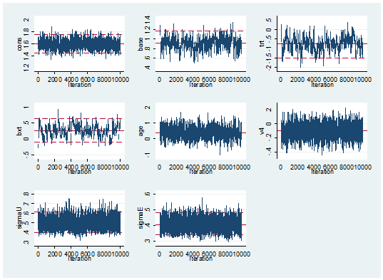
----------------------------------------------------------
 Parameter n    mean    sd    sem median     95% CrI
 ---------------------------------------------------------
 cons   10000  1.598 0.077 0.0029  1.598 ( 1.450, 1.754 )
 base   10000  0.909 0.131 0.0086  0.909 ( 0.640, 1.167 )
 trt    10000 -0.765 0.363 0.0325 -0.766 ( -1.500, -0.068 )
 bxt    10000  0.259 0.188 0.0242  0.260 ( -0.107, 0.631 )
 age    10000  0.383 0.351 0.0134  0.380 ( -0.286, 1.074 )
 v4     10000 -0.100 0.090 0.0019 -0.099 ( -0.276, 0.079 )
 sigmaU 10000  0.495 0.055 0.0007  0.491 ( 0.397, 0.615 )
 sigmaE 10000  0.406 0.036 0.0006  0.404 ( 0.338, 0.482 )
 ----------------------------------------------------------
On the whole not my best day.
The mixing is a disappointment but the run time is not a real surprise.
The problem with this algorithm is that we exchange 4×59=236 Poisson counts for 2184 augmented times; that is, 236 plus the total number of events. On top of that we need a further 2184 augmented identifiers for the mixture components. Not only do we have to simulate these values but then we have to include them in the calculations for the Gibbs sampler.
It has to be said that the long run time was acknowledged in the original technical report that I referred to in the previous posting and because of this, the same authors devised another augmentation algorithm based on just two times for each Poisson observation; the very last interval and the total time before the last observed event. Since the total time is the sum of exponentials it does not have an exponential distribution and we have to use another mixture to approximate that density.
I am currently rather disillusioned with data augmentation and I’ve decided not to bother.
The reference for anyone who wants to try the faster augmentation algorithm is,
Fruhwirth-Schnatter S, Fruhwirth R, Held L and Rue H
Improved auxiliary mixture sampling for hierarchical models of non-Gaussian data
Stat Comput 2009;19:479-492
Poor mixing is inherent in any algorithm that updates one parameter at a time whenever the parameters are correlated and this holds even when we use a Gibbs sampler to sample from the correct conditional distributions. In a couple of weeks time I am going to discuss Stan, an alternative to WinBUGS that, it is claimed, will perform well even when Gibbs sampling struggles.
As usual the code for my Mata program can be downloaded from my web page at https://www2.le.ac.uk/Members/trj

 Subscribe to John's posts
Recent Comments