Poisson regression with two random effects: MCMC by data augmentation

When I restarted this blog after the Christmas break I resolved to concentrate more on straightforward applications of Bayesian analysis with Stata; I believe that is what most Stata users are interested in. A couple of months in and I am going to ignore my good intensions and discuss a topic that I considered too advanced to mention in my book, namely MCMC by data augmentation.

The idea is simple even if its application is sometimes involved; to simplify the MCMC algorithm we look to see if there are any extra data, that, if only we had them, would make the analysis much simpler. Then we treat those data as being missing or unobserved and we add an extra stage to the analysis. In stage 1 we simulate the unobserved data, and in stage 2 we use the simulated values of the unobserved data to solve the problem. The calculation involves two stages instead of one, but if the two stages are both quick then we might still have a very efficient algorithm.

Let’s put this method into symbols; y is the original data and z is the additional, unobserved data and ultimately we want the posterior p(θ|y).
p(θ|y) α ∫ p(θ|y,z) p(z|θ,y) dz
Sampling θ directly from p(θ|y) may be hard but if it is easy to sample the unobserved data z from p(z|θ,y) and it is easy to sample θ from p(θ|y,z) then we are on to a winner.

The addition of unobserved data is usually called data augmentation and whether or not it works well is problem dependent. Sometimes we can spot a good augmentation and sometimes we can’t.

The problem of data augmentation for generalized linear models with random effects has been well-studied and there are some quite neat augmentation algorithms for those models. In fact, data augmentation is the basis of the JAGS glm module that so dramatically improved the performance of JAGS for our Poisson regression problem.

The theory
There is a well-known result concerning Poisson distributions that we will need. This states that if events occur at random with a fixed rate then the number of events in a specified time will follow a Poisson distribution and the lengths of the intervals between successive events will follow an exponential distribution.

With the epilepsy data we know the number of seizures a subject has in a 2 week period but we do not have the exact times of the seizures. Those exact times will be our unobserved data and the unobserved times between the seizures will have an exponential distribution.

Actually it turns out that it is easier to work with the log of the times between the seizures. So we will need the distribution of the log of an exponential variable.

Approximating the density
Using the change of variables method discussed in section 2.9 of Bayesian Analysis with Stata it is not difficult to show that if t ~ exponential(λ) so that its density is p(t) = exp(-t/λ)/λ, then the density of x=log(t/λ) is p(x) = exp(x-exp(x)). As is my usual practice I have put the mathematics in a pdf called augmentation for those who want the details.

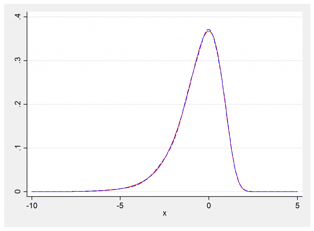
So we will need the likelihood of the distribution p(x) = exp(x-exp(x)). One way to get this is to approximate it by a mixture of normal distributions. Individual normal distributions are easy to handle and mixtures of normal distributions are not much more complicated. Here is some Stata code that shows the density exp(x-exp(x)) and a 5 component normal mixture that approximates it quite closely.

range x -10 5 1000
gen f = exp(x-exp(x))
gen y = 0.2924*normalden(x,0.0982,0.4900) ///
     + 0.2599*normalden(x,-1.5320,1.0896) ///
     + 0.2480*normalden(x,-0.7433,0.6150) ///
     + 0.1525*normalden(x,0.8303,0.4382) ///
     + 0.0472*normalden(x,-3.1428,1.7993)
twoway (line f x, col(red)) (line y x, col(blue)), leg(off)

The actual distribution is shown in red and the normal mixture is shown as a blue dashed line. The approximation is really very impressive and plenty good enough for an MCMC algorithm.

The constants in the mixture distribution are taken from a technical report by Sylvia Fruhwirth-Schnatter and Helga Wagner (http://www.jku.at/ifas/content/e108280/e146255/e146306/ifasrp04_2004.pdf). They are the researchers who developed this method.

Simulating the unobserved data
The next step is to consider how we might simulate the unobserved times of the seizures conditional on knowing how many there were (y) and the current estimate of the rate (μ).

Let’s assume that μ is the expected number of events in a 2 week period and we want to express the times as a proportion of that period, i.e. as numbers between (0,1). For illustration we will consider someone who has three seizures, y=3.

Since the events in a Poisson process are completely random we could generate the times of the three seizures by taking three uniform(0,1) random numbers e.g. 0.451, 0.325, 0.772
Sort them in ascending order gives 0.325, 0.451, 0.772 and the intervals are
0.325, 0.126, 0.321
The interval up to the end of the period is 0.228 but at that time we have not yet seen the next seizure so the full interval will be at least 0.228.

We can generate exponential intervals using –log(u)/ μ , where u is another uniform(0,1) variable and completely random processes have no memory so a random exponential interval that is at least 0.228 long can be simulated using 0.228- log(u)/μ. Let’s suppose that we end up with four intervals
0.325, 0.126, 0.321, 0.630
These are the simulated values of the augmented or unobserved data that I will call t.

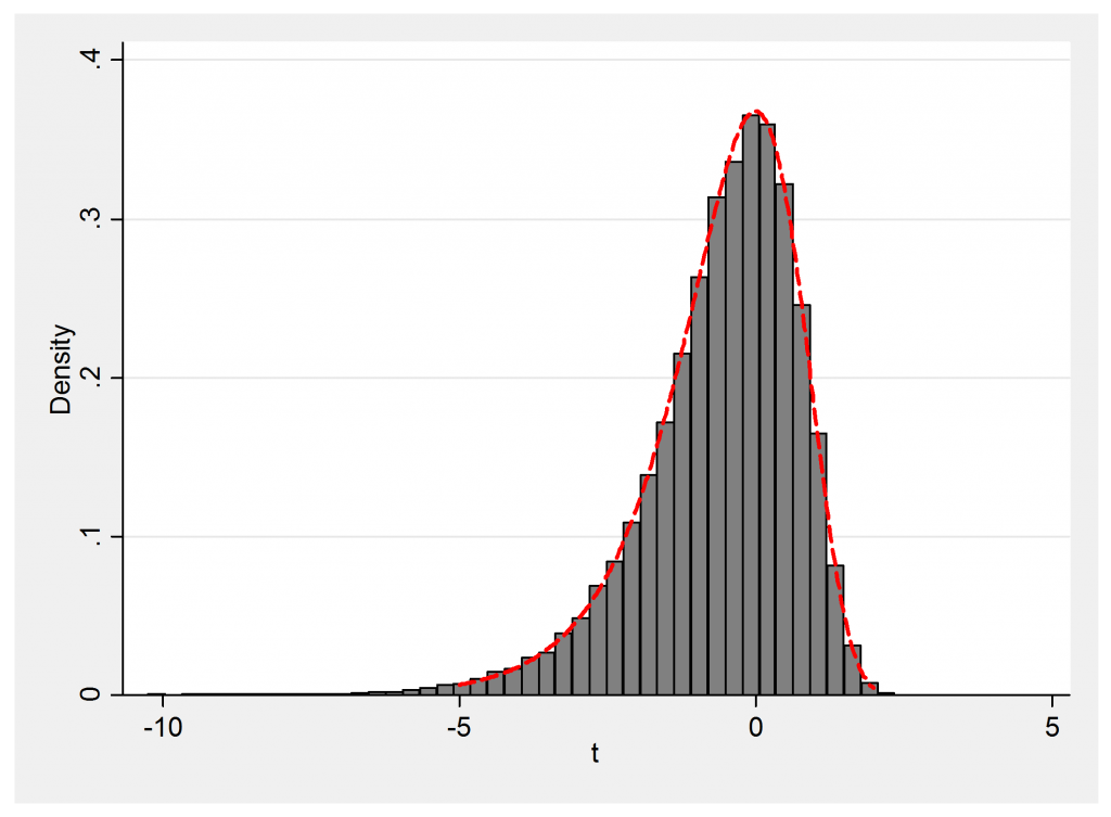
Let’s demonstrate that t sampled in this way does follow the distribution p(ε) = exp(ε -exp(ε)).

clear
 tempname pf
postfile `pf’ t using temp.dta, replace
local mu = 5
local theta = log(`mu’)
forvalues iter=1/5000 {
     local n = rpoisson(`mu’)
     drop _all
     if `n’ == 0 {
          local t = 1 – log(runiform())/exp(`theta’)
          local t = log(`t’) + `theta’
          post `pf’ (`t’)
     }
    else {
          local m = `n’ + 1
          qui set obs `m’
          qui gen u = 0 in 1
          qui replace u = runiform() in 2/`m’
          sort u
          qui gen t = u[_n+1]-u
          qui replace t = 1 – u[`m’] – log(runiform())/exp(`theta’) in `m’
          qui replace t = log(t) + `theta’
          forvalues i=1/`m’ {
               post `pf’ (t[`i’])
          }
     }
}
postclose `pf’
use temp.dta, clear

histogram t , density addplot( function y = exp(x-exp(x)) , range(-5 2) lwid(0.5) lcol(red) ) leg(off)

Again there is very close agreement between theory and simulation.

Selecting one component from the mixture
So far we have seen that for Poisson data with rate μ, the intervals between events will be exponential with mean λ=1/μ and
log t = log λ + ε = -log μ + ε
where ε is a variable from the distribution p(ε) = exp(ε -exp(ε)) , which we can approximate with a mixture of 5 normal distributions.

One more step. The normal mixture is made up of 5 normal distributions. Life would be much simpler if we knew which of the five components our particular ε comes from, so let’s make that information part of the unobserved data. Call it r, which will be a integer between 1 and 5. Simulate r  and then
log t = -log μ + e
were e comes from the rth normal distribution in the mixture.

Given all of the unobserved data, the model is just a simple normal errors regression and provided that we choose conjugate priors we can solve this very easily with a Gibbs sampler. So our problem is solved in three stages
1. Simulate the intervals between the events, t
2. Simulate the number of the component from the mixture, r
3. Fit the normal errors model by Gibbs sampling

The three stages are all quick and should mix well, potentially much better that running a Metropolis-Hastings algorithm for the original problem.

There are a couple of points that I have jumped over, such as how to generate r and how to write the Gibbs sampler but those too are simple and the first is described in the pdf augmentation and the second will be the subject of my next posting.

Enough for one week; after Easter I will program this algorithm in Mata and see how it performs when we analyse the epilepsy data.