In the previous posting in this series on RJMCMC, I created a Stata program for the following problem.
We have two binomial samples y1=8, n1=20 and y2=16, n2=30, but we are not sure whether to model them as,
M1: binomials with different probabilities π1 and π2
M2: binomials with a common probability ξ.
For my priors I chose, p(M1)=0.3 and p(M2)=0.7. Under M1 my priors on the parameters were p(π1|M1)=Beta(5,5) and p(π2|M1)=Beta(10,10) and under M2, p(η|M2)=Beta(20,20).
In the previous programs we imagined a vector of parameters Ψ with two elements (Ψ1,Ψ2). When we selected model M1 we just set π1=Ψ1 and π2=Ψ2. While when in model M2 we set ξ=Ψ1 and created an arbitrarily distributed, unused parameter u=Ψ2. I then set up a Metropolis-Hastings algorithm to control switches between the models and everything worked well.
It turned out that the posterior probability of M2 is about 0.77, only slightly higher than our prior model probability. So the data move us slightly in the direction of model 2. The posterior distribution of the binomial probabilities when in model 1 has a mean for π1=0.433 and π2=0.520 and under model 2 the posterior mean for ξ=0.489.
This algorithm represents a rather special case of RJMCMC because it does not involve any transformations when we move between Ψ and the particular parameters of the two models, or if you wish you can say that there is a transformation but it takes the form of a simple equality. The result is that the Jacobians of the transformations are 1 and we can leave them out of the calculations.
What I want to do now is to introduce a transformation into the algorithm so that we are forced to calculate the Jacobians.
First let me present again the Stata program for RJMCMC without transformation. This is effectively the same as the program that we had before, except that I have expanded the code slightly with a few redundant calculations intended to prepare us for the generalization needed when we incorporate transformations.
program myRJMCMC
args logpost b ipar
local M = `b'[1,1]
if( runiform() < 0.5 ) {
* update within the current model
if( `M’ == 1 ) {
local pi1 = rbeta(13,17)
local pi2 = rbeta(26,24)
local psi1 = `pi1′
local psi2 = `pi2′
}
else {
local xi = rbeta(44,46)
local u = rbeta(1,1)
local psi1 = `xi’
local psi2 = `u’
}
matrix `b'[1,2] = `psi1′
matrix `b'[1,3] = `psi2′
}
else {
* try to switch
local psi1 = `b'[1,2]
local psi2 = `b'[1,3]
local pi1 = `psi1′
local pi2 = `psi2′
local xi = `psi1′
local u = `psi2′
local a1 = log(binomialp(20,8,`pi1′))+log(binomialp(30,16,`pi2′))+ ///
log(betaden(5,5,`pi1′))+log(betaden(10,10,`pi2′))+log(0.3)
local a2 = log(binomialp(20,8,`xi’))+log(binomialp(30,16,`xi’))+ ///
log(betaden(20,20,`xi’))+log(betaden(1,1,`u’))+log(0.7)
if `M’ == 1 {
if log(runiform()) < `a2′ – `a1′ matrix `b'[1,1] = 2
}
else {
if log(runiform()) < `a1′ – `a2′ matrix `b'[1,1] = 1
}
}
end
matrix b = (1, 0.5, 0.5)
mcmcrun logpost b using temp.csv , replace ///
param(m psi1 psi2) burn(500) update(20000) thin(2) ///
samplers( myRJMCMC , dim(3) )
insheet using temp.csv, clear
gen pi1 = psi1
gen pi2 = psi2
mcmcstats pi1 pi2 if m == 1
gen xi = psi1
gen u = psi2
mcmcstats xi u if m == 2
tabulate m
The main features of the program are:
(a) randomly with probability 0.5, I decide either to update the parameters within the current model or to propose a move between models
(b) the within model updates are able to use Gibbs sampling because we have chosen conjugate priors
(c) the MH algorithm for switching between models calculates the acceptance probability from the likelihood of the data under that model, the prior on the parameters under that model, the prior model probability and the probability of selecting that move. Calculations are performed on a log-scale to avoid loss of precision due to very small quantities.
(d) The chance of proposing a move to M2 when we are in M1 is the same as the chance of proposing a model to M1 when we are in M2 (i.e. 0.5) so these probabilities cancel and I have left them out of the acceptance probabilities.
(e) the distribution of M2’s unused parameter, u, is arbitrary. Here it is Beta(1,1) which is a very poor choice given that under the other model the equivalent parameter is Beta(26,24). This will have a small impact on mixing but the algorithm will recover and give the correct posterior.
Now let us introduce a transformation into the algorithm. Under model 2, ξ is a common binomial parameter that replaces the separate binomial probabilities π1 and π2. So a natural idea would be make ξ equal to the average of π1 and π2. We could write this as,
Under M1
π1 = Ψ1
π2 = Ψ2
Under M2
ξ = (Ψ1+Ψ2)/2
u = Ψ2
A word of warning before we continue. In the paper in The American Statistician from which I took this problem, they use a very similar transformation, in fact they use a weighted average instead of a simple average. However, as we will see, transformations based on any sort of average cause problems and the algorithm breaks down under extreme conditions. So this is a nice illustration of RJMCMC partly because it fails and we can discover why it fails. Perhaps you can already see from the formulae for the transformations why we are going to run into difficulties.
A couple of weeks ago we derived the formula for the MH acceptance probability as
f(Y|Ψ,Mk) f(Ψ|Mk) dΨ P(Mk) g(Mk to Mj) / f(Y|Ψ,Mj) f(Ψ|Mj) dΨ P(Mj) g(Mj to Mk)
Each product in the ratio includes a likelihood, a prior on the parameters, a prior on the model and the probability of selecting that move. The extra term is dΨ is present to turn the density of the prior into a probability.
We are going to work in terms of π1 and π2 or ξ and u and so we will need to transform the dΨ’s into small elements, dπ1 and dπ2 or dξ and du this means multiplying by the Jacobian formed from derivatives dπ1/dΨ etc.
In our program we calculate the MH acceptance probabilities with the lines
local a1 = log(binomialp(20,8,`pi1′))+log(binomialp(30,16,`pi2′))+ ///
log(betaden(5,5,`pi1′))+log(betaden(10,10,`pi2′))+log(0.3)
local a2 = log(binomialp(20,8,`xi’))+log(binomialp(30,16,`xi’))+ ///
log(betaden(20,20,`xi’))+log(betaden(1,1,`u’))+log(0.7)
The initial transformations both had a Jacobian of 1 because they were based on equalities with derivatives of 1 and, of course, the log(1) is zero so I did not bother to include the Jacobians in the code.
The new transformation for M2 has the form
ξ = (Ψ1+Ψ2)/2
u = Ψ2
So the matrix of derivatives dξ/Ψ1 ,dξ/Ψ2, du/Ψ1, du/dΨ2 has the form
0.5 0.5
0 1
which has determinant 0.5. This is our Jacobian. It says that small increments on the dξ scale are half the size of the corresponding increments on the dΨ1 scale.
Noting that out transformation implies that Ψ1=2ξ-u, we can modify our Stata code. The changes are in red.
program myRJMCMC
args logpost b ipar
local M = `b'[1,1]
if( runiform() < 0.5 ) {
* update within the current model
if( `M’ == 1 ) {
local pi1 = rbeta(13,17)
local pi2 = rbeta(26,24)
local psi1 = `pi1′
local psi2 = `pi2′
}
else {
local xi = rbeta(44,46)
local u = rbeta(1,1)
local psi1 = 2*`xi’-`u’
local psi2 = `u’
}
matrix `b'[1,2] = `psi1′
matrix `b'[1,3] = `psi2′
}
else {
* try to switch
local psi1 = `b'[1,2]
local psi2 = `b'[1,3]
local pi1 = `psi1′
local pi2 = `psi2′
local xi = (`psi1’+`psi2′)/2
local u = `psi2′
local a1 = log(binomialp(20,8,`pi1′))+log(binomialp(30,16,`pi2′))+ ///
log(betaden(5,5,`pi1′))+log(betaden(10,10,`pi2′))+log(0.3)
local a2 = log(binomialp(20,8,`xi’))+log(binomialp(30,16,`xi’))+ ///
log(betaden(20,20,`xi’))+log(betaden(1,1,`u’))+log(0.7)+log(0.5)
if `M’ == 1 {
if log(runiform()) < `a2′ – `a1′ matrix `b'[1,1] = 2
}
else {
if log(runiform()) < `a1′ – `a2′ matrix `b'[1,1] = 1
}
}
end
As I warned earlier this is almost correct but not quite and it fails to give the correct model posterior as it spends too much time in model 1.
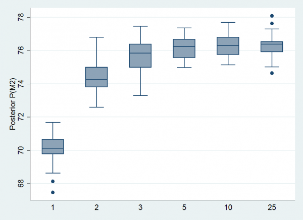
To illustrate the breakdown of the algorithm, I ran this program with different priors for u ranging between Beta(25,25), Beta(10,10), Beta(5,5), Beta(3,3), Beta(2,2) and Beta(1,1). Each time I ran the algorithm for 10,000 iterations and repeated the analysis 25 times. The number of iterations is rather on the low side so we get quite a bit of sampling error between the 25 repeat runs. Here is a boxplot of the estimates of the mean posterior probability for Model 2 plotted on a percentage scale.
Our previous analysis showed that the correct answer is just under 77%. So we get reasonable, but not perfect, estimates when we use Beta(25,25) as our prior for u but the estimates deteriorate markedly when we use Beta(1,1). Yet the theory says that the prior on u is arbitrary.
Beta(1,1) is equivalent to a uniform distribution, so occasionally under model M2 we might generate a value 0.95 for u. Suppose, at the same time, we generate ξ=0.45 then we will calculate Ψ1=2ξ-u=-0.05 and when we propose a move to model M1, we will set π1=-0.05 and we are in trouble because π1 is a probability and it must be between 0 and 1.
Our choice of making ξ the average would be a sensible transformation if there were no constraints on the parameters but when the parameters must all lie in (0,1), it will sometimes fail. Now when we use Beta(25,25) this problem does not arise very often because there is such a small probability of picking an extreme value for u and so we stay in the region where the elements of Ψ are both between 0 and 1.
It is more complicated, but much better to use the transformation
Under M1
π1 = invlogit(Ψ1)
π2 = invlogit(Ψ2)
Under M2
ξ = (invlogit(Ψ1)+invlogit(Ψ2))/2
u = invlogit(Ψ2)
In this set up, the elements of Ψ are unconstrained and can take any value between -∞ and ∞ and, whatever those values, they always transform to π1 and π2 or ξ and u that are between 0 and 1. As before, we need derivatives such as dξ/Ψ1 and dξ/Ψ2 although, in this case, the algebra is marginally easier if we calculate dΨ1/dξ and the use the relationship dξ/Ψ1 = 1/ (dΨ1/dξ).
Let’s start with M1 and invert the transformation.
Ψ1 = logit(π1) = log( π1/(1-π1))
Ψ2 = logit(π2) = log( π2/(1-π2))
So dΨ1/dπ1 = 1/[π1(1-π1)] and inverting this formula we obtain dπ1/dΨ1 = π1(1-π1) which means that the Jacobian matrix is
π1(1-π1) 0
0 π2(1-π2)
and the determinant is π1(1-π1)π2(1-π2)
Similar calculations show that the Jacobian for model 2 is ξ(1-ξ)u(1-u)/2.
Now we can write a much better RJMCMC program.
program myRJMCMC
args logpost b ipar
local M = `b'[1,1]
if( runiform() < 0.5 ) {
* update within the current model
if( `M’ == 1 ) {
local pi1 = rbeta(13,17)
local pi2 = rbeta(26,24)
local psi1 = logit(`pi1′)
local psi2 = logit(`pi2′)
}
else {
local xi = rbeta(44,46)
local u = rbeta(1,1)
local psi1 = 2*logit(`xi’)-logit(`u’)
local psi2 = logit(`u’)
}
matrix `b'[1,2] = `psi1′
matrix `b'[1,3] = `psi2′
}
else {
* try to switch
local psi1 = `b'[1,2]
local psi2 = `b'[1,3]
local pi1 = invlogit(`psi1′)
local pi2 = invlogit(`psi2′)
local xi = (invlogit(`psi1′)+invlogit(`psi2′))/2
local u = invlogit(`psi2′)
local J1 = `pi1’*(1-`pi1′)*`pi2’*(1 -`pi2′)
local J2 = `xi’*(1-`xi’)*`u’*(1-`u’)/2
local a1 = log(binomialp(20,8,`pi1′))+log(binomialp(30,16,`pi2′))+ ///
log(betaden(5,5,`pi1′))+log(betaden(10,10,`pi2′))+log(0.3)+log(`J1′)
local a2 = log(binomialp(20,8,`xi’))+log(binomialp(30,16,`xi’))+ ///
log(betaden(20,20,`xi’))+log(betaden(1,1,`u’))+log(0.7)+log(`J2′)
if `M’ == 1 {
if log(runiform()) < `a2′ – `a1′ matrix `b'[1,1] = 2
}
else {
if log(runiform()) < `a1′ – `a2′ matrix `b'[1,1] = 1
}
}
end
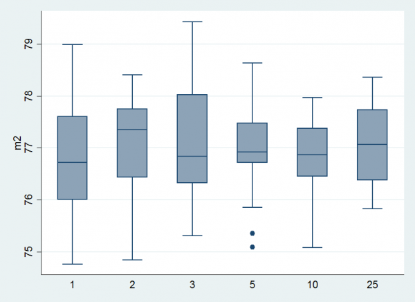
I ran this program for a the same range of priors on u and obtained the results.
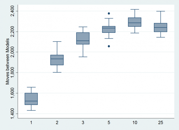
It is clear that the mean estimate does not depend on u but the variation between repeat runs is larger when we use Beta(1,1) because we make fewer moves between models.
Here is a boxplot of the numbers of model switches per run of 10,000 iterations. Beta(10,10) looks best.
Before finishing I should point out that Peter Green’s original version of RJMCMC is very slightly different to the formulation that I have presented.
Suppose that we have a large set of alternative models that can require anything between 1 and 20 parameters. We are currently in a model that requires 3 parameters and we propose a move to a model with 5 parameters. We do not need to worry about the 15 parameters that neither model requires. In other words instead of defining a full set of parameters, Ψ, we can work with the reduced set that covers the two models that we are currently comparing. This is more efficient but it requires slightly more complicated programming. In my opinion, it is both easier to follow and easier to code if we always return to the full set of parameters.
I think that we have done this example to death. Now we need to move on to more complex applications such as the flu epidemic analysis that started us on the RJMCMC path.


 Subscribe to John's posts
Recent Comments