Using R with Stata: Part II

This is the second in a series of posting about conducting advanced statistical analyses in Stata by sending a job to R and then reading the results back into Stata. Our task for testing this process is to use the R package, DPpackage, to fit a Bayesian Dirichlet process mixture (DPM) model for smoothing a scatter plot. The data that we are using consist of 298 IgG measurements made on children of different ages.

In my last posting I described the R code needed to fit the model and this time I will consider how that code can be submitted and run without leaving Stata.

Let us first assume that we have a text file called DPC.R than contains the R script. Repeating what we had last time, the file will contain,

setwd(‘E:/IGG’)
require(foreign)
require(DPpackage)
D <- read.dta(‘igg.dta’)
zbar <- c(7,3)
Sigma <- matrix(c(4,1,1,1),2,2)
MyPrior <- list(alpha=5, k0=0.25, nu1=10, m1=zbar, psiinv1=7*solve(Sigma))
MyDesign <- list(nburn=5000, nsave=5000, nskip=3, ndisplay=1000)
xp ← c(1,2,3,4,5)
fitIgG <- DPcdensity(y=D$igg, x=D$age, xpred=xp,ngrid=100,
compute.band=TRUE, type.band=”HPD”, prior=MyPrior, mcmc=MyDesign,
state=NULL, status=TRUE)
nClu <- as.data.frame(fitIgG$save.state$thetasave[,7])
names(nClu) <- “nclus”
write.dta(nClu,file=’nclusters.dta’)
cDen <- as.data.frame(cbind(fitIgG$grid,t(rbind(fitIgG$densp.m,
fitIgG$densp.l,fitIgG$densp.h))))
names(cDen) <- c(“IgG”,”m1″,”m2″,”m3″,”m4”,”m5”,
“l1″,”l2″,”l3″,”l4″,”l5″,”h1″,”h2″,”h3″,”h4″,”h5”)
write.dta(cDen,file=’cDensity.dta’)

Having created this text file, we can send it to R using Stata’s shell command. For instance, if we were to type the Stata command,
. shell notepad

Stata would be suspended while the operating system opens the notepad text editor. Stata would become active again when notepad is closed.

When R is installed from http://www.r-project.org/ (R is free), a bin directory  is created that will include a file called R.exe. Within Stata, we can run the R script from file DPC.R if we type,
. shell path/R.exe CMD BATCH DPC.R log.txt

where the word path is replaced by the full path to R.exe on your computer. This command will suspend Stata while R runs the script as a batch job (it might take a few minutes). R sends its output, including any error messages to the log file. We can subsequently inspect this log file within Stata using,
. type log.txt

Now I run several different programs in this way and it is tedious to have to remember the path to each program so I store them in a file called executables.txt, which is saved in my PERSONAL directory.

Here is a listing of the first 5 lines of my file executables.txt.

PLINK,”C:\Software\PLINK\plink.exe”
FBAT,”C:\Software\fbat\fbat202C_win\fbat.exe”
R,”C:\Program Files\R\R-3.0.2\bin\x64\R.exe”
WINBUGS,”C:\Software\WinBUGS14\WinBUGS14.exe”
OPENBUGS,”C:\Software\OpenBUGS\OpenBUGS.exe”

The file contains the name of each program that I use, a comma, and then the path.

Matched to this file I have an ado file called execute.ado that reads the required path from this file and runs the executable. The contents of execute.ado are

program execute
gettoken PG CD : 0
local personal : sysdir PERSONAL
tempname fh
file open `fh’ using `personal’executables.txt ,read
file read `fh’ inLine
while !r(eof) {
tokenize `”`inLine'”‘, parse(“,”)
if upper(“`1′”) == “`PG'” local executable “`3′”
file read `fh’ inLine
}
file close `fh’
confirm file “`executable'”
shell “`executable'” `CD’
end

So we could give Stata the command
. execute R CMD BATCH DPC.R log.txt
and execute.ado would locate the appropriate path for R and ‘shell’ it together with the remainder of the command line.

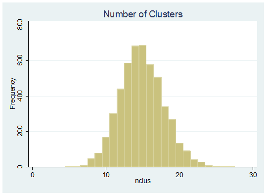
Our R script not only runs DPcdensity but it returns some of the output as Stata .dta files so after it has run we might plot a histogram of the number of cluster in each of the 5,000 stored iterations of the sampler.

. use nclusters.dta, clear
. histogram nclus , start(0.5) width(1) freq title(Number of Clusters)

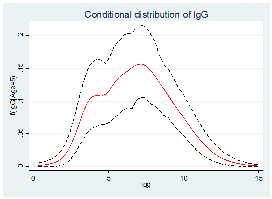
Alternatively we could plot the conditional distribution at age 5 years using,

. use cDensity.dta, clear
. twoway (line m5 igg , lpat(solid) lcol(red)) ///
       (line l5 igg , lpat(dash) lcol(black)) ///
       (line h5 igg , lpat(dash) lcol(black)), ///
       leg(off) title(Conditional distribution of IgG) ytitle(f(IgG|Age=5))

This method can be adapted for any R analysis but it has one severe limitation. To use it, you must be able to program in R. This is fine for my own work, but is not very helpful if I am collaborating with someone who is not an experienced R programmer.

Next time I will describe how I make the facilities of R available within Stata for people who do not know how to program R. The approach involves writing a Stata ado file that creates the R script as well as running it. In this way a Stata user only needs to install R on their computer, they do not need to know anything of its programming language.