Smoothing a scatter plot

In my last posting I mentioned that in is possible to use Stata to run R packages by preparing an R script, calling R from within Stata so that R runs in the background and then reading R’s results into Stata for further processing. The big advantage of this method is that one does not need to  re-write the R package in order to make its analysis available in Stata. To illustrate this process I will analyse some data using a Bayesian scatter plot smoother that is available in an R package called DPpackage.

Before I use this R package, I’ll introduce the statistical problem by describing a simpler Bayesian scatter plot smoother implemented entirely in Stata.

Some time ago I showed how to fit Bayesian finite mixture models in Stata and I introduced a program called mixmnormal (https://staffblogs.le.ac.uk/bayeswithstata/2014/05/09/mixtures-of-normal-distributions/); now we will adapt that program to smooth a scatter plot. The idea behind this use of mixture models dates back at least to Muller et al (Biometrika 1996;83:67-79) who described how to use an infinite normal mixture as a scatter plot smoother. R’s DPpackage implements Muller’s method, but this week I will use a large, but finite, mixture, in order to obtain an approximation to that method.

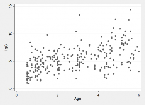
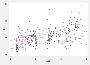
To illustrate the method I will use some data on the concentration of Immunoglobin G (IgG) measured in a sample of 298 children aged under 6 years. IgG is a component of the immune system and can be found in the blood and other body fluids. It binds to the surfaces of bacteria and viruses, immobilizing them and enabling phagocytic cells to recognise them. The normal range in adults is between 7 and 15 g/L but in children the normal range is lower and varies with age. The data were used by Nuofaily and Jones (Applied Statistics 2013;62:723-740) to illustrate quantile regression based on a generalized gamma distribution.

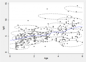
The idea behind the mixture method is to approximate the two-dimensional distribution of points by a finite mixture of normal distributions, as in the following illustration.

We can draw a slice through the mixture at a chosen age and obtain a flexible approximation to the conditional distribution by combining the component distributions. Alternatively we can find the conditional expectation, E(y|x), for any chosen age, x, by combining the conditional means of each of the components.

The fitted trend line is just the average of these expectations weighted by the probability of a point falling in that component and the probability of the particular x for that component. Repeating this calculation for lots of x’s enables us to draw the smooth trend line, shown in blue in the illustration.

In the code below the priors and initial values are set and then the Bayesian mixture fitting program fits the model. The priors are set using the local r to denote the number of components in the mixture.

 local r = 20
 matrix R = J(2,2*`r',0)
 forvalues j=1/`r' {
     matrix R[1,2*`j'-1] = 4
     matrix R[2,2*`j'] = 4
 }
 matrix df = J(1,`r',16)
 matrix M = J(2,`r',4)
 matrix B = J(2,2*`r',0)
 forvalues j=1/`r' {
     matrix B[1,2*`j'-1] = 0.1
     matrix B[2,2*`j'] = 0.1
 }
 matrix ALPHA = J(1,`r',40/`r')
 matrix T = J(2,2*`r',0)
 forvalues j=1/`r' {
    matrix T[1,2*`j'-1] = 1
    matrix T[2,2*`j'] = 1
 }
 matrix C = J(298,1,1)
 forvalues i=1/298 {
     matrix C[`i',1] = 1 + int(20*runiform())
 }
 matrix P = J(1,`r',1/`r')
 matrix MU = M
 mixmnormal igg age, mu(MU) t(T) p(P) n(`r') m(M) b(B) r(R) ///
     df(df) c(C) alpha(ALPHA) ///
     burnin(1000) updates(5000) filename("igg.csv")

Now we can calculate the expectations and average them across the iterations. The chain of 5000 updates is thinned by taking every 10th from iteration 5 onwards in order to save time in the calculation.

 local r = 20
 insheet using igg.csv, clear
 merge 1:1 _n using igg.dta
 range x 0 6 1001
 foreach iter of numlist 5(10)5000 {
     qui gen e`iter' = 0 in 1/1001
     qui gen w = 0 in 1/1001
     forvalues s=1/`r' {
         matrix T = J(2,2,0)
         matrix T[1,1] = t`s'_1_1[`iter']
         matrix T[2,1] = t`s'_2_1[`iter']
         matrix T[1,2] = t`s'_1_2[`iter']
         matrix T[2,2] = t`s'_2_2[`iter']
         matrix V = syminv(T)
         local sy = sqrt(V[1,1])
         local sx = sqrt(V[2,2])
         local rho = V[1,2]/(`sy'*`sx')
         local my = mu`s'_1[`iter']
         local mx = mu`s'_2[`iter']
         local p = p`s'[`iter']
         qui replace e`iter' = e`iter' + `p'*(`my'+`rho'*`sy'* ///
            (x - `mx')/`sx')*normalden((x - `mx')/`sx')
         qui replace w = w + `p'*normalden((x - `mx')/`sx')
     }
     qui replace e`iter' = e`iter'/w
     drop w
 }
 egen fmean = rowmean(e*)
 egen fp10 = rowpctile(e*) , p(10)
 gen fp10 = rowpctile(e*) , p(90)
 twoway (scatter igg age) (line fmean x, lpat(solid) lcol(red)) ///
   (line fp10 x, lpat(dash) lcol(blue)) (line fp90 x, lpat(dash) ///
   lcol(blue)), leg(off) xtitle(Age) ytitle(IgG)

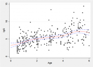
Because we have a simulated Bayesian model fit it is a simple matter to find the average trend line and the 10% and 90% quantiles shown in red and blue in the plot below.

The choice of the number of components and setting of the priors together control the degree of smoothing and care should be taken when chosing these values. Perhaps by trying out different choices on simulated data to gain a feel for the degree of smoothing produced by a given set of priors.

In the paper by Noufaily and Jones the authors set themselves the slightly different problem of estimating the quantiles of the sample rather than smoothing the scatter plot. The fitted mixture model can be used to address this problem as well.

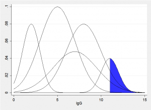
Imagine a vertical slice though the fitted bivariate components corresponding to some value x, we would obtain something similar to the picture below. The sum of these normal distributions produces represents the fitted conditional distribution for a particular age. The quantile that excludes q% will have q% of the sum of the areas in the blue region. All we need to do is to try a range of trial values of IgG until we find the value that excludes the required amount.

Below is a plot of the 10th, 25th, 50th, 75th and 90th quantiles. The code requires looping over lots of values of x so takes a few minutes to run and is given at the end of this posting. With relatively little effort this could be incorporated into an ado file in order to automate the entire analysis.

Next time I will analyse the same data using a Bayesian infinite mixture model with Dirichlet process priors fitted by R’s DPpackage but controlled and run from within Stata.

Code for performing quantile regression based on a fitted mixture distribution,

local r = 20
 insheet using igg.csv, clear
 merge 1:1 _n using igg.dta
 local n = 61
 range x 0 6 61
 range y 0 15 1001
 gen Q10 = 0
 gen Q25 = 0
 gen Q50 = 0
 gen Q75 = 0
 gen Q90 = 0
 forvalues k=1/61 {
 local x = x[`k']
 local nIter = 0
 foreach iter of numlist 5(50)5000 {
 local ++nIter
 qui gen q = 0 in 1/1001
 qui gen w = 0 in 1/1001
 forvalues s=1/`r' {
 matrix T = J(2,2,0)
 matrix T[1,1] = t`s'_1_1[`iter']
 matrix T[2,1] = t`s'_2_1[`iter']
 matrix T[1,2] = t`s'_1_2[`iter']
 matrix T[2,2] = t`s'_2_2[`iter']
 matrix V = syminv(T)
 local sy = sqrt(V[1,1])
 local sx = sqrt(V[2,2])
 local rho = V[1,2]/(`sy'*`sx')
 local my = mu`s'_1[`iter']
 local mx = mu`s'_2[`iter']
 local p = p`s'[`iter']
 qui replace q = q + `p'*normal( (y-(`my'+`rho'*`sy'*(`x' - `mx')/ ////
 `sx'))/(`sy'*sqrt(1-`rho'*`rho')) )*normalden((`x' - `mx')/`sx')
 qui replace w = w + `p'*normalden((`x' - `mx')/`sx')
 }
 qui replace q = q/w
 drop w
 qui replace q = 0.1 in 1002
 qui replace q = 0.25 in 1003
 qui replace q = 0.5 in 1004
 qui replace q = 0.75 in 1005
 qui replace q = 0.9 in 1006
 qui ipolate y q , gen(iy)
 qui replace Q10 = Q10 + iy[1002] in `k'
 qui replace Q25 = Q25 + iy[1003] in `k'
 qui replace Q50 = Q50 + iy[1004] in `k'
 qui replace Q75 = Q75 + iy[1005] in `k'
 qui replace Q90 = Q90 + iy[1006] in `k'
 drop iy q
 }
 }
 qui replace Q10 = Q10/`nIter'
 qui replace Q25 = Q25/`nIter'
 qui replace Q50 = Q50/`nIter'
 qui replace Q75 = Q75/`nIter'
 qui replace Q90 = Q90/`nIter'
 twoway (scatter igg age) (line Q10 x, lpat(dot) lcol(blue)) ///
 (line Q25 x, lpat(dash) lcol(blue)) (line Q50 x, lpat(solid) lcol(red)) ///
 (line Q75 x, lpat(dash) lcol(blue)) (line Q90 x, lpat(dot) lcol(blue)), ///
 leg(off) xtitle(Age) ytitle(IgG)