Mixtures of Normal Distributions

In my last posting I started a library of Mata functions for use in Bayesian and this week I will add a function that fits mixtures of normal distribution using a Bayesian Gibbs sampling algorithm.

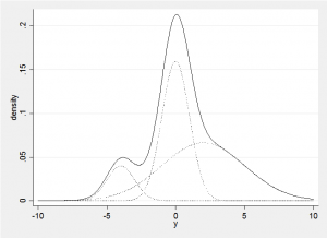
The normal distribution is the underlying assumption for many statistical models and data are often transformed to make their distribution look normal so that these standard methods can be used. When we cannot find an appropriate transformation to normality, we are forced to consider other distributions with a more appropriate shape, but the theory behind analyses that use non-normal distributions is often appreciably more complex. One way to maintain the nice mathematical properties of the normal distribution but to gain far greater flexibility of shape is to mix together two or more normal distributions. The example below shows how a non-symmetrical distribution with two modes and a heavy tail can be formed from a mixture of three normal distributions.

This mixture distribution is made up of a set of component normal distributions and we can generalize this approach into higher dimensions in a simple Bayesian analysis provided that we are willing to use multivariate normal priors for the means of the components, Wishart priors for the precision matrices of the components and a Dirichlet prior for the proportions from each component. Under these conditions all of the distributions will be conjugate and it is trivial to derive a Gibbs sampler for fitting the model. The algorithm starts with initial parameter estimates and an initial allocation of subjects/items to the components and then the algorithm cycles repeatedly through 4 steps:

1. Update the mean for each component normal distribution using data on the subjects currently allocated to that component
2. Update the variance matrix for each component using data on subjects currently allocated to that component
3. Update the probabilities of belonging to each component using the current numbers allocated to each component
4. Update the allocation of subjects to components using the probabilities that a person’s data would be generated by each component

My Mata function that implements this Gibbs sampler is called mixMNormal() and has been added to the library libbayes and instructions for downloading it are given at the end of this posting. The general method for creating libbayes was discussed in a previous posting, ‘Creating a Mata Library’.

The function, mixMNormal(), needs to able to cope with any number of components, each with its own precision matrix but unfortunately Mata does not allow arrays of matrices. My solution is to pack the matrices into one large matrix by adding them to the right. So suppose that we have bivariate data so that the precision matrices Ti are all 2×2 and let’s imagine that there are three components in the mixture, so i=1,2,3. The three precision matrices are packed into a 2×6 matrix as T=[T1,T2,T3].

To unpack the matrices we can use Mata’s powerful range indexing. In which T[|1,3\2,4|] extracts the matrix with top left element (1,3) and bottom right element (2,4). In our example with would extract T2 from T.

Finally if you look at the code for  mixMNormal() you will see that it writes the parameter estimates from each update to a comma delimited file so they can be read back into Stata using the -insheet- or –import– commands. There is no equivalent of the -post- command in Mata that would write directly to a .dta file.

An unfortunate feature of Mata is that were the program to crash (it shouldn’t but you never know), or should you stop the run before it has finished, then the comma delimited results file will be left open and any future attempt to use that file name during the current session will result in an error (the file is only closed when you close Stata). As far as I know there is no other way to close such an open file, so to continue you must select a fresh name for the csv file.

To use the Mata function from within Stata it is convenient to create a Stata program that calls mixMNormal(). You could make this very elaborate by, for instance, adding the facility for if or in, or making data checks for missing data, or checks on the sizes of matrices; however, the following code does the basic job.

program mixmnormal 

   syntax varlist , MU(string) T(string) P(string) n(integer) ///

       M(string) B(string) R(string) DF(string) C(string) ALPHA(string) ///

       BUrnin(integer) Updates(integer) Filename(string)

   tempname Y

   mata: mata clear

   qui putmata `Y'=(`varlist')

   local list "`mu' `r' `df' `m' `b' `t' `c' `alpha' `p'"

   foreach item of local list {

     mata : `item' = st_matrix("`item'")

   }

   cap erase "`filename'"

   mata: mixMNormal(`Y',`mu',`t',`p',`n',`m',`b',`r',`df', \\\

     `c',`alpha',`burnin',`updates',"`filename'")

end 

This code copies the data and the matrices from Stata’s memory into Mata’s memory and then calls mixMNormal(). It is included in the download file referred to at the end of the posting for anyone who wants to try it.

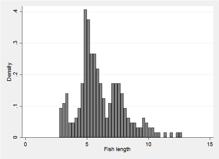
Although the code works with any dimension of data we will return to one dimension for the example since this is easier to visualize. We will model the distribution of fish lengths given in a much analysed data set referred to in the book by Titterington et al Statistical analysis of finite mixture distributions Wiley 1985 and subsequently supplied in the R package bayesmix. The data set contains the lengths (presumably in inches) of 256 snappers.

In our first analysis we will fit a mixture with 6 components and set the parameter for the Dirichlet prior to (20,20,10,5,1,1). Thus we can think of our prior knowledge as being equivalent to having a previous sample of 57 fish in which we found two common components, two rare components and two in between. Given that there are only 256 fish in the actual data, this prior will be equivalent to about 1/5 of the data.

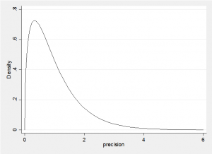
In the absence of real knowledge about the locations of the components, we will set the priors on the means to all be Normal with mean 6 and precision=0.1. That is the prior on the component means has a standard deviation of 3.2=1/sqrt(0.1) so we expect the components to have means in the approximate range (0,12). Finally we must place a prior on the precision of each component. In one dimension a Wishart W(R,k) is equivalent to a Gamma distribution G(k/2,2/R) so it has mean precision of k/R, or put another way, a variance of R/k. If we set k=3 and R=3, then we expect the components to have a standard deviation of 1, but the distribution of the precision would be

So we would not be surprised by a precision of 0.25 (st dev=2) or a precision of 4 (st dev=0.5). What this prior will do, is avoid components with very small standard deviations, so it will tend to avoid fitting a component to a single fish.

Putting this together we have

matrix R = (3,3,3,3,3,3)

matrix df = (3,3,3,3,3,3)

matrix M = (6,6,6,6,6,6)

matrix B = (0.1,0.1,0.1,0.1,0.1,0.1)

matrix ALPHA = (20,20,10,5,1,1)

The initial values are not critical provided that we run a long enough burnin. I chose,

matrix T = (1,1,1,1,1,1)

matrix C = J(256,1,1)

forvalues i=1/256 {

   matrix C[`i',1] = 1 + int(6*runiform())

}

matrix P = J(1,6,1/6)

matrix MU = M

 

Then I ran a burnin of 2500 before plotting five fitted curves 1000 iterations apart

mixmnormal fish , mu(MU) t(T) p(P) n(6) m(M) b(B) r(R) ///

   df(df) c(C) alpha(ALPHA) ///

   burnin(2500) updates(5000) filename(temp.csv)

insheet using temp.csv, clear

set obs 1001

range y 0 15 1001

foreach iter of numlist 1000 2000 3000 4000 5000 {

   gen f`iter' = 0

   forvalues s=1/6 {

   qui replace f`iter' = f`iter' + p`s'[`iter']* /// 

     normalden(y,mu`s'_1[`iter'],1/sqrt(t`s'_1_1[`iter']))

   }

}

merge 1:1 _n using fish.dta

histogram fish , start(2) width(0.25) xtitle(Fish length) ///

   addplot((line f1000 y, lpat(solid) lcol(blue)) ///

   (line f2000 y, lpat(solid) lcol(red)) ///

   (line f3000 y, lpat(solid) lcol(green)) ///

   (line f4000 y, lpat(solid) lcol(black)) ///

   (line f5000 y, lpat(solid) lcol(orange)) ) leg(off)

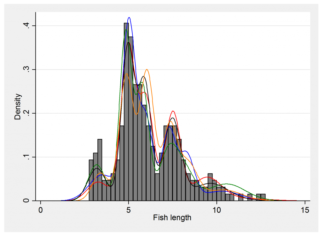
The coloured lines show the uncertainty in the model fit and are taken from 5 different points in the chain. Presumably these components correspond to fish of different ages that have grown to different sizes.

The table of mean parameter estimates is:

Component	Percentage	Mean	sd
1	10%	3.4	0.50
2	32%	5.0	0.36
3	24%	5.9	0.82
4	19%	7.4	0.48
5	10%	9.5	0.82
6	3%	10.8	0.94

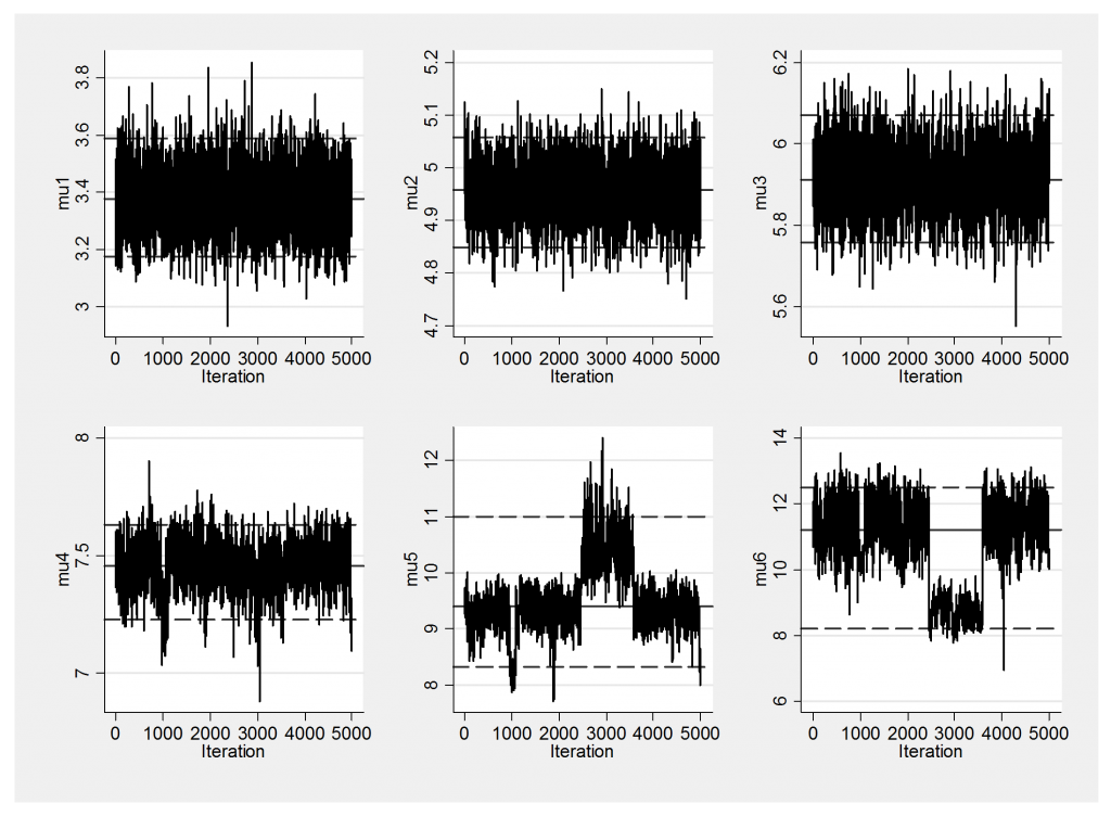
Notice that now both components 5 and 6 have relatively large standard deviations and that these standard deviations are big enough that the bumps centred on the corresponding means will tend to overlap. Keeping this in mind let us look at the trace plot of the 5000 simulations.

The solutions for the first 4 components are quite stable but because the last two overlap slightly the algorithm cannot decide whether to call the component with mean 9, number 5, and the component with mean 11, number 6, or to label them the other way around. In fact it jumps between the two solutions at about simulation 2500 and then jumps back again about a 1,000 simulations later. It even looks as if another brief switch took place at around iteration 1,000 that also affected component 4. Because of this label switching it is not sensible to take the average of mu5 and call it the mean of a component; mu5 actually represents different component means at different times.

I think that I will return to the problem of label switching in my next posting. Meanwhile if you would like to try this analysis for yourself, the code that I used can be downloaded from fishPrograms.