In my previous posting, I discussed a coursework that I set my students on the use of Stata’s –ml– command and I suggested that a Bayesian analysis of the same problem using Stata would raises a few interesting issues. Now I would like to start to address those points.
To recap briefly, the idea of the problem is that viral load, a measure of the severity of an infection, can be measured in different body fluids and the logs of two such viral loads can be modelled by a bivariate normal distribution. The assay used to measure viral load has a minimum level of detection and so for a significant proportion of subjects, one or both of these levels will be undetectable. The earlier posting includes some references and describes the data.
With no missing data and conjugate priors for the mean and covariance structure of the bivariate normal, we could create a very fast Gibbs sampling algorithm for fitting the model. The data that are missing because of the limit of detection add very little to the complexity because we can treat each missing value as another parameter to be estimated by the Gibbs sampler.
To analyse the data in WinBUGS would require use of the censoring operator I(,) with a multivariate normal distribution and unfortunately this is not allowed. I keep thinking of different ways of tricking WinBUGS into fitting this model but so far none of them has worked. So I will program the Gibbs sampler directly in Stata. This is straightforward except for two small problems.
- The conjugate prior for a precision matrix is the Wishart distribution and Stata does not have a built in function for generating random values from a Wishart.
- We will need a way of simulating values from a truncated bivariate normal distribution.
So we must briefly consider these two issues before presenting the Gibbs sampler.
The do file for the Gibbs Sampler is available for download and you can try it for yourself if you wish. The instructions for downloading it are given at the end of this posting.
Wishart Distribution
One way to sample from the Wishart is to use the Bartlett decomposition as described on Wikipedia (http://en.wikipedia.org/wiki/Conjugate_prior ). It only requires methods for simulating values from univariate normal and chi-squared distributions, both of which are available in Stata.
Truncated Normal variables
The Stata command –drawnorm– simulates values from a multivariate normal distribution when there is no truncation but I have chosen to write my own program as this is marginally faster.
To simulate a value from a truncated univariate normal N(m,s) when it is known that the value must lie in the range (-inf,K), we need
local Y = `m’+ invnorm(runiform()*normal((`K’-`m’)/`s’))*`s’
In this code, we calculate the proportion, normal((`K’-`m’)/`s’), of the distribution that lies inside the allowed interval and then take a random proportion of that amount and convert it back onto the normal scale using the invnormal() function.
For a bivariate normal distribution we can factorize so that
f(y1,y2) = f(y2|y1) f(y1)
and then if y1 lies in (-inf,K1) and y2 lies in (-inf,K2)
local Y1 = `m1’+ invnorm(runiform()*normal((`K1′-`m1′)/`s1′))*`s1′
local m21 = `m2’ + `r’*`s2’*(`Y1’-`m1’)/`s1’
local s21 = `s2’*sqrt(1-`r’*`r’)
local Y2 = `m21’+ invnorm(runiform()*normal((`K2′-`m21′)/`s21′))*`s21′
Here m21 and s21 are the mean and standard deviation of the condition distribution of Y2 given Y1. (http://en.wikipedia.org/wiki/Multivariate_normal_distribution )
The Gibbs Sampler
The algebra for the conjugate analysis of a Multivariate Normal distribution is already available on countless websites, see for example (http://en.wikipedia.org/wiki/Conjugate_prior ).
My program is called viralGibbs.do and it successively updates the mean, precision matrix and then the missing values. I create the chain with the house-keeping program –mcmcrun-, which I introduce in my book, ‘Bayesian Analysis with Stata’. This command controls the sampling and stores the updates, so all I need to do is to make sure that viralGibbs.do has the arguments that mcmcrun expects. When using general samplers such as Metropolis-Hastings or adaptive rejection, the first argument would be the name of a program that calculates the log-posterior, but in a Gibbs sampler we don’t need this function so in my code it is replaced by a dummy. The second argument is the row vector, b, containing the parameters. I have chosen to place 6 parameters in b, namely the means, variances, covariance of the bivariate normal and also, rather arbitrarily and for illustration, the estimate for the missing value corresponding to the 9th saliva measurement.
To run this program we must first set the priors and initial values. As you will see if you look at the do file, my priors were influenced by the study of Shepard et al described in my previous posting, though in truth they are pretty vague since I was not confident that the results from one assay on a particular sample would carry over to a different assay used on people who had had different treatments.
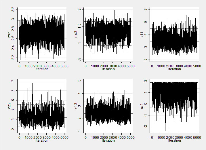
Mixing and convergence are very good so a short burnin (1000) and run (5000) are all that is required. Here is a trace plot of the simulations which shows good mixing.
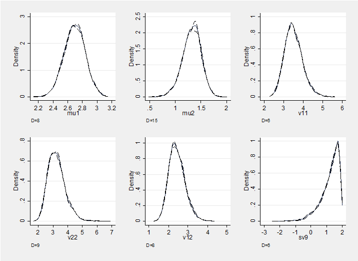
and here is a section plot of the chain which also supports convergence. The plot shows density estimates for the marginal posterior distributions of the six parameters together with density estimates based on the first and second halves of the chain; these densities are almost indistinguishable.
Here are the results as summarised by my downloadable Stata command –mcmcstats-
----------------------------------------------------------------------------
Parameter n mean sd sem median 95% CrI
----------------------------------------------------------------------------
mu1 5000 2.693 0.144 0.0023 2.694 ( 2.407, 2.977 )
mu2 5000 1.321 0.182 0.0045 1.332 ( 0.929, 1.649 )
v11 5000 3.505 0.457 0.0102 3.468 ( 2.705, 4.511 )
v12 5000 2.440 0.416 0.0104 2.400 ( 1.731, 3.348 )
v22 5000 3.257 0.595 0.0198 3.199 ( 2.300, 4.586 )
sv9 5000 1.216 0.590 0.0085 1.374 ( -0.282, 1.876 )
s1 5000 1.868 0.121 0.0027 1.862 ( 1.645, 2.124 )
s2 5000 1.798 0.162 0.0054 1.788 ( 1.516, 2.141 )
r 5000 0.722 0.046 0.0011 0.724 ( 0.624, 0.804 )
----------------------------------------------------------------------------
The posterior means are very similar to the maximum likelihood estimates that my students were required to find using -ml- and which are given in Chu et al (Applied Statistics 2005;54:831-845) although those authors did not use Stata. The MLEs for the means are (2.64,1.32) and for the standard deviations (1.88,1.74) and correlation 0.73. Likewise the confidence intervals from the likelihood analysis are very similar to the Bayesian credible intervals reflecting the vagueness of my priors.
Downloading the Stata code
You can net install the commands mcmcrun, mcmcstats, mcmctrace and mcmcsection all of which are described in ‘Bayesian analysis with Stata’ from http://stata-press.com/data/bas
Until the book is actually published, these files should be treated as being still under test but as far as I know they are fine to use. The Stata code and data for this particular analysis can be downloaded from here as a pdf file viralGibbs; you would need to copy and paste the contents into a do-file and a data file. The book is due to be published shortly, but in the meantime you might find my manual helpful. It can also be downloaded from here manual.


 Subscribe to John's posts
Recent Comments