Why I don’t use WinBUGS priors

In the WinBUGS help system there are a number of worked examples that have been very influential in shaping the way that people perform Bayesian analysis. Those examples use very vague priors, such as a normal distribution with a mean of zero and standard deviation of a thousand. Many people have learned to use Bayesian methods by copying those examples and so they have tended to adopt the same approach to their priors. I have never liked vague priors of the type adopted by WinBUGS and I am going to try to explain why I did not use them in the book ‘Bayesian analysis with Stata’.

The case for WinBUGS priors

The argument, as it has been put to me, is that very vague priors will have a minimal influence on the analysis and will allow the data to dominate. The prior may not be realistic but the likelihood will dictate the range of plausible parameter values and the vague prior will be virtually flat over that range. Similar vague priors have been used so many times that they have become a widely accepted standard and they make it easier to compare the results from analyses based on different models. There is the added, usually unspoken, advantage that if we always use N(0,sd=1000) we do not need to spend time eliciting true priors.

WinBUGS priors are unrealistic

We cannot talk about realism without taking specific examples, so let’s start with the WinBUGS worked example called DUDONGS. The data consist of measurements of the lengths, in metres, of sea-cows. There is a parameter alpha in the model that represents an upper limit on the lengths of a group of sea-cows of different ages. The prior for this parameter is taken to be N(0,sd=1000). Now you may not know much about the size of a dudong, but I doubt if you would really want to place half of your prior probability on the length being negative. This prior also places substantial amounts of probability on lengths up to about 2000m and once again you probably don’t really believe that they can grow that big. In fact a moment spend on Wikipedia will tell you that sea-cows rarely grow to be over 3 metres and the largest ever found was about 4 metres long.

Vagueness is scale dependent

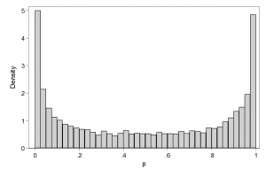
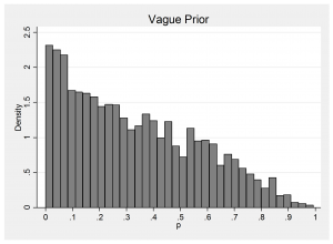
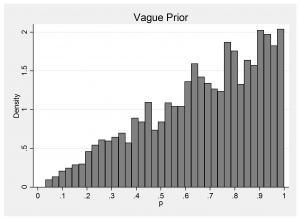
BLOCKER is a WinBUGS example that analyses some data on mortality in different clinical trials of beta-blockers. Mortality in the control group is modelled such that the logit of the probability of death has a prior that is N(0,sd=316). Since there is no information to distinguish the individual trials, this same prior was used for each one. This prior is flat over a wide range of logits but what about the implied prior for the probability of death? In fact, the prior is so extreme that it is difficult to picture, so let us look at N(0,sd=3.16) instead. The implied prior on the probability of dying in the control group is,

The corresponding picture for N(0,316) just looks like two spikes at 0 and 1 with a tiny amount of probability fairly evenly spread between the peaks.

We may get away with this choice of prior because a clinical trial will be designed to be large enough to measure the probability of death in the control group quite accurately, but if we used such a prior with sparse data it would be highly informative.

Does it matter?

Let us consider an example of the use of a vague prior in combination with some sparse data. We will take the case of a binomial model for data generated with p=0.3 and n=3. So in the experiment we will observe one of the possibe results, y=0, 1, 2 or 3 with probabilities 0.34, 0.44, 0.19, 0.03.

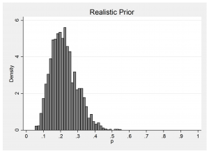
We will place a normal prior on the logit scale and either make mu=logit(p) very vague, mu ~N(0,300) as in a WinBUGS example or make it realistic, mu ~ N(-1.4,0.5). The WinBUGS style prior, as we have already seen, places two spikes at p=0 and p=1 with a small amount of probability fairly evenly spread in between and my realistical prior represents the beliefs of someone who thinks that p will be about 0.2 and who would be surprised if p were under 0.08 or over 0.4. Here is a plot of the implied realistic prior on p.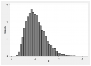

This prior is certainly not vague. On the p scale, the standard deviation is about 0.1 so it resembles the distribution that you would get from a binomial sample of about n=20 observations (sqrt(0.3×0.7/n)=0.1).

The ‘realistic’ prior is centred in the wrong place but then so is the vague prior. The critical difference is that the realistic prior wrongly prefers 0.2 to 0.3 while the vague prior treats those two values more or less equally. Indeed the vague prior gives more or less equal belief to all plausible values of p.

When we collect the data, 44% of the time y will equal 1 and the posteriors under the two models will be,

and 19% of the time y=2 and the posteriors will be,

34% of the time y=0 and the realistic prior gives

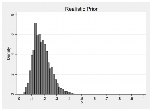and the vague prior causes my program to crash. I used a Metropolis-Hastings algorithm and it tried to make p approach 0, so mu moved towards minus infinity and went beyond the precision of my computer.

3% of the time y=3 and a similar problem occurs. The vague prior crashes as mu gets large while the realistic prior gives,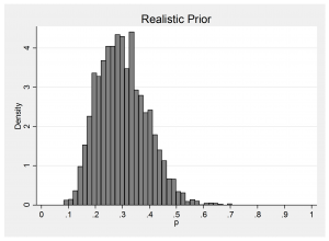

I would argue that in all of the four possible situations, the analysis under the realistic prior is preferable.

It may never happen

Those members of the ostrich tendency are probably thinking that the example is extreme and that these problems don’t occur in practice. It is true that it is easy to see what has gone wrong with this example (that is why I chose it) and most statisticians would be able to foresee the difficulty, or at least spot it after the event and change the prior (i.e. produce a dishonest analysis).

But what about a complex model with a hierarchical structure and lots of correlated parameters? Will you ever be sure that none of the parameters is effectively dependent on a few of the observations and so would be poorly estimated? Perhaps, this is why your complex WinBUGS program crashes or is very slow to converge.

What should we do?

I think that the answer is obvious. We should use realistic priors. When the data are sparse, the estimates will still be realistic and when we have lots of data, our prior will have little influence. So in the binomial example I opted for N(-1.4,0.5) but if I were less confident about by guess that p=0.2, I could have gone for N(-1.4,1) which would have concentrated my belief over the range 0.03 to 0.65 instead of 0.08 to 0.4. Perhaps you are not happy with either of these choices, in which case you could make the prior even more vague, or you could centre it somewhere else, or you could give it a different shape. The point is that it is important that you think about the prior and choose something realistic that you are happy with and not simply opt for unrealistic, vague priors just because you have seen them used in the WinBUGS manual.