
On the internet there is a host of sites that describe the mathematics of Dirichlet processes, but very few of them try to explain the ideas behind the algebra. Dirichlet process methods are very important for modern Bayesian analysis and raise a number of interesting programming issues when they are to be implemented in Stata, but I thought that before getting too involved in the technicalities, it would be useful to try to explain the logic behind the mathematics.
The Bayesian method tells us how to update our beliefs about the parameters of a statistical model, so there can be no such thing as a Bayesian analysis without parameters. Despite this, the literature is full of articles describing, so called, non-parametric Bayesian methods. Clearly there is a problem of terminology. The irony is that when a Bayesian talks of a non-parametric analysis what they actually mean is, an analysis based on a very flexible model with a large, possibly infinite, number of parameters.
In its broadest sense non-parametric Bayesian analysis includes models that, for instance, use splines to create flexible curves to represent the trend in the data, but more frequently the term is used to refer to methods based on very flexible distributions.
In Bayesian analysis the most widely used method for creating a flexible family of distributions is based on the Dirichlet distribution, or to be more exact its infinite cousin the Dirichlet Process. Eventually, I should like to develop some Stata programs for Bayesian analysis that avoid assuming standard distributional families such as the normal or gamma but replace them with Dirichlet processes.
A typical situation in which we might want flexibility arises when we use a hierarchical or random effects model. Perhaps we have a multi-centre study and we want to place a distribution over the centre effects, as if the centres were a random sample from all of the centres that might have been included in the study. Standard methods require us to assume that the centre effects have a normal distribution, but such an assumption is often very hard to justify, so we might prefer a more flexible distribution such as that provided by a Dirichlet process.
The Dirichlet Distribution
Since a Dirichlet process is just an infinite version of the Dirichlet distribution, let’s start by recapping some of the basics of that distribution and to make things concrete I will take a simple example.
When we look at generic variants at a particular location on the DNA, we usually record the genotype, that is, the count of the number of the rare form of the variant that an individual carries. Since we all have chromosomes in pairs, we can have 0, 1 or 2 copies of any variant. Over a population we can describe the frequency of such genotypes in terms of three probabilities p0, p1 and p2.
Let’s suppose that we want to estimate the three genotype probabilities from a sample of 40 people of whom 20 have no copies of the rarer variant, 10 have 1 copy and 10 have 2 copies. In the absence of any other information the best estimates would be ½, ¼, ¼ but of course, as good Bayesians, we know that we are never in that situation.
Over the last decade many millions of pounds have been spend studying genetic variants and there will be a wealth of information on our variant available through any one of numerous internet databases. Let’s suppose that studies of this variant in similar populations suggest that the genotypes usually occur in the ratio 6:3:1 and we would like an analysis that incorporates this prior information.
If our 40 subjects are unrelated and randomly drawn from the population, then the distribution of the genotype counts will be multinomial, that is,
p(data|parameters) α p020 p110 p210
A convenient (conjugate) prior for these probabilities is the Dirichlet,
p(parameters) α p0a0-1 p1a1-1 p2a2-1
So this Dirichlet distribution has three parameters a0, a1 and a2 that we must choose in such a way that the distribution reflects our prior beliefs. The properties of the Dirichlet are described in detail on Wikipedia at http://en.wikipedia.org/wiki/Dirichlet_distribution and perhaps the most important fact is that under this distribution E(pj) = aj/sum(a’s), so an easy way to present our prior beliefs would be to choose a0=6, a1=3 and a2=1 then E(p0)=0.6 etc.
The conjugate property of the Dirichlet with the multinomial means that all of the Bayesian calculations are trivial and our posterior beliefs would be described by
Dir(6+20, 3+10,1+10)
I have already described a simple algorithm for generating Dir(6,3,1) random variables from gamma variables https://staffblogs.le.ac.uk/bayeswithstata/2014/05/02/creating-a-mata-library/; in Stata we can use the code
. gen g0 = rgamma(6,1)
. gen g1 = rgamma(3,1)
. gen g2 = rgamma(1,1)
. gen p0 = g0/(g0+g1+g2)
. gen p1 = g1/(g0+g1+g2)
. gen p2 = g2/(g0+g1+g2)
So we can generate random samples from the prior Dir(6,3,1) and the posterior Dir(26,13,11) and find the marginal distributions pictured below.
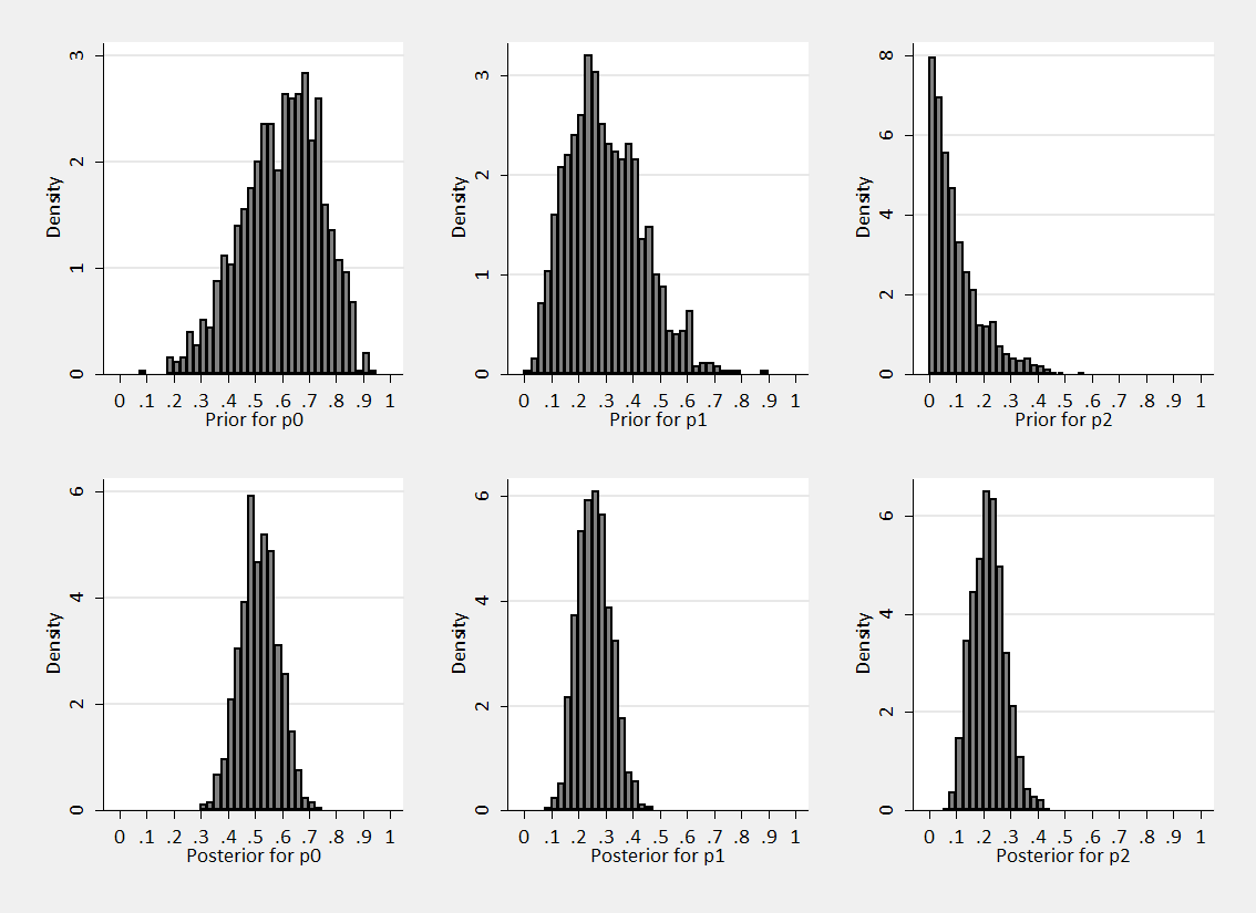
We can see that the data push us towards the solution ½, ¼, ¼ .
However we had we been stronger in our prior beliefs we could have set a0=18, a1=9 and a2=3. The ratios are the same, so we would have had the same expectations E(p0)=0.6 etc. The priors and posteriors would now be
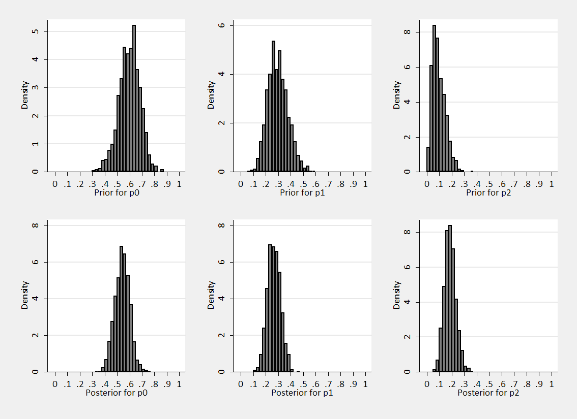
As we might expect, the increase in prior information leads to narrower posteriors and posteriors centred closer to the prior means.
An alternative way to write Dir(6,3,1) and Dir(18,9,3) is as Dir(10;0.6,0.3,0.1) and Dir(30;0.6,0.3,0.1); this format emphasises that they both have the same expectations but different strengths of prior belief. The parameter that controls the strength of our beliefs is sometimes called the concentration parameter.
In this formulation let’s suppose that our prior is Dir(M;f0,f1,f2) and we have n0 observations equal to 0, n1 equal to 1 and n2 equal to 2 (so N=n0+n1+n2). The posterior will be
Dir(M+N;(Mf0+n0)/(M+N), (Mf1+n1)/(M+N), (Mf2+n2)/(M+N)).
The concentration parameter increases by the number of observations and the expectations are weighted averages of the prior and the data.
Data Simulation
Now let us suppose that we want to generate a sample of 10 values X1,…X10 representing the genotypes of 10 people when the genotype probabilities have a Dir(30;0.6,0.3,0.1) prior distribution.
Algorithm 1: Via the p’s
(a) Generate p0, p1 and p2 from Dir(30;0.6,0.3,0.1)
(b) Use p0,p1,p2 to create an independent multinomial sample of size 10.
For example, in a particular simulation you might get (0.62,0.34,0.04) as the probabilities and then (0,0,1,0,0,0,2,0,0,1) as the sample of data. You could repeat this lots of times drawing fresh probabilities and fresh data each time.
Algorithm 2: The Chinese Restaurant
For i=1…10
With probability 30/(30+i-1)
draw Xi to be 0,1 or 2 with probabilities equal to the prior expectations (0.6,0.3,0.1)
Otherwise
select a random integer j between 1 and i-1 and set Xi = Xj
So this algorithm draws the X’s from a mixture distribution, either we repeat a value that has already been sampled or we generate a new value from the expectations of the prior. The more data we already have, the more likely we are to repeat an existing value.
To persuade you that these are equivalent without a heap of mathematics, I have written a Stata program that simulates values by the two methods and then compares summaries of the simulated data. You can download it here (TwoAlgorithms).
So the algorithms are equivalent, who cares? Algorithm2 is both more complex and slower to run, however it has one big advantage. We get the sample of X’s without ever simulating the probabilities p0, p1, p2. This advantage is irrelevant when we have a simple Dirichlet distribution, but we want to generalize to a Dirichlet process with an infinite number of probabilities. In the infinite case it will not be possible to use Algorithm 1 but Algorithm 2 will still work.
In the infinite case, algorithm 2 is sometimes called the Chinese restaurant process since it is said that it mirrors what happens when someone walks into a restaurant and either recognises a friend and joins them at their table or they choose their table at random. Not a helpful analogy in my view.
The Chinese restaurant algorithm is clever but it can lead to a misunderstanding. When it is used, we hide the intermediate stage that is dependent on the probabilities. It is easy therefore to fall into the trap of thinking that the Dirichlet distribution is a model for the data, when in fact it is a prior distribution on the probabilities and it is those probabilities that define the model for the data.
In my next posting I will move from the Dirichlet distribution with its finite number of parameters to the very flexible Dirichlet process with an infinite number of parameters and from there I will move on to develop some Stata programs for non-parameteric Bayesian analysis.

 Subscribe to John's posts
Recent Comments