Last week I discussed Google Flu Trends a project that provided weekly estimates of the number of flu cases in 25 different countries based on the frequency of internet searches for influenza related terms (https://en.wikipedia.org/wiki/Google_Flu_Trends). Sadly Google have stopped producing these estimates but historical data are still available for download. Presumably Google gave up when faced with criticism of the accuracy of the method. Much of that criticism appears to have been fuelled by a general unease about the use of ‘big data’, anyway I hope that it did not come from statisticians, who should be familiar with measurement error and surrogates.
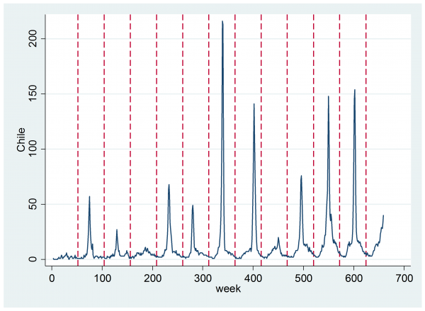
The plot below shows the estimates of the number of flu cases each week for Chile. The vertical lines denote periods of 52 weeks. As Chile is in the southern hemisphere, the winter peak in flu cases occurs around the middle of the year.

The pattern seems to be, an annual cycle that is almost zero at the start and end of the year, on to which is imposed an annual spike corresponding to a flu epidemic. These spikes are of varying severity and duration. Perhaps there is also a drift upwards in the total number of estimated cases per year, which I suppose to be a result of increased internet use rather than a genuine increase in the number of flu cases, though the latter is not impossible given a growing population and increased urbanisation.
Anyway, our aim is to model these data in such a way that enables us to determine the starts of the annual epidemics. To that end, in my last posting I developed a Metropolis-Hastings sampler called mhsint that updates integer based parameters, such as the week in which an epidemic starts or the week when it ends. What we need now is a Bayesian model for these data.
The model that I am going to adopt just follows my description. I will suppose that the counts follow a Poisson distribution and that the log of the mean number of cases has a linear drift over time plus a sine term that has a frequency of π/52 (≈0.06), so that it rises and falls back to zero over 52 weeks
log(mean) = a + b time/1000 + c sin(0.060415*week)
On top of this basic trend I’ll impose an annual epidemic of strength Hi that starts in week Si and ends in week Ei, where i denotes the year. So
log(mean) = a + b time/1000 + c sin(0.060415*week)+Hi δ(year==i & week>=Si & week<=Ei)
Here δ is 0 or 1 depending on whether the condition holds.
Preparing the data
The data can be downloaded from https://www.google.org/flutrends/about/ by clicking on world or the country that interests you. There is a parallel dataset for Dengue Fever. I copied the portion of the file that contains the data and since it is comma delimited, I saved it as a .csv file that I called googleflu.csv.
A little preprocessing is required to turn dates into week numbers and to drop incomplete years. Eventually we obtain, year=1…12 corresponding to 2003…2014, week = 1…52 or 53 (it depends when the first day of the first week falls in that year) and time = 1…627 denoting the week number.
insheet using googleflu.csv , clear
gen day = date(date,”YMD”)
gen time = 1+(day-day[1])/7
gen year = real(substr(date,1,4))
gen start = year != year[_n-1]
gen t = start*time
sort year time
by year: egen w = sum(t)
gen week = time – w + 1
drop w t start
drop if year==2002 | year==2015
drop if chile == .
replace year = year – 2002
keep year week time chile
save tempflu.dta, replace
Priors
The intercept parameter, called a in my model formula, represents the log of the predicted number of cases at the start of the first year when it is the height of the Chilean summer, I’ll suppose that a ~ N(0,sd=1). A value of 0 would correspond to an expectation of 1 case per week.
I’ve scaled the time by dividing by 1000 because I expect the trend per week to be very small. If the coefficient b were 1 then after 1000 weeks (≈20 years) the predicted number of cases would have drifted up by a factor of about 3. I’ll suppose that b ~ N(1,sd=1)
Each year the sine term goes from 0 to a peak of 1 and back to 0. In the absence of an epidemic I would imagine that the background predicted number of cases might increase by a factor of perhaps 10 between the summer and the winter, so I’ll make the coefficient of the sine term, c ~ N(2,sd=1).
As to the the extent of the epidemics, I imagine that they might increase the background rate by a factor of 10 or even 100, but an epidemic cannot lower the number of cases, so Hi must all be positive. I’ll make Hi ~ Gamma(2,0.5)
It is more difficult to place a prior on the start and end of an epidemic because Si and Ei will not be independent. I’ll suppose that the epidemic is likely to start around week 20 and make
P(Si=k) α 1/(1+abs(k-20)) Si < 1 & Si < 50
and
P(Ei=h|Si=k) α 1/(1+abs(h-k-8)) Ei>Si & Ei<=52
which would imply that I expect the epidemic to last 8 weeks.
Calculating the log-posterior
The code for calculating the log-posterior follows the description of the model. The only places where we must be careful are when guarding against an invalid model. This can happen when the limits of the epidemic move outside [1,52], or when the epidemic ends before it starts, or when the value of the log-posterior becomes infinite.
It is an unfortunate aspect of Stata that infinity is represented by a large positive number so any time that the log-posterior become infinite, the Metropolis-Hastings algorithm will automatically accept the move. In this model, this can happen if we try a very large value for the severity of the spike because the log-posterior depends on the exponential of this value and scalars in Stata can only go up to about 10300 before they exceed the double precision of a computer.
In the following code, the parameters are arranged in a row matrix, b, so that a, b and c come first, then the 12 Hi‘s the the 12 Si‘s and finally the 12 Eis.
program logpost
args lnf b
local invalid = 0
tempvar eta lnL
gen `eta’ = `b'[1,1]+`b'[1,2]*time/1000+`b'[1,3]*sin(0.060415*week)
local hterm = 0
forvalues i=1/12 {
local h = `b'[1,`i’+3]
local hterm = log(`h’) – 2*`h’
local S = `b'[1,`i’+15]
local E = `b'[1,`i’+27]
if `E’ <= `S’ | `E’ > 52 | `S’ < 2 | `h’ > 250 local invalid = 1
local hterm = `hterm’ – log(1+abs(`S’-20)) – log(1+abs(`E’-`S’-8))
replace `eta’ = `eta’ + `h’ if year == `i’ & week >= `S’ & week <= `E’ }
if `invalid’ == 1 scalar `lnf’ = -9e300
else {
gen `lnL’ = chile*`eta’ – exp(`eta’)
qui su `lnL’
scalar `lnf’ = r(sum) + `hterm’ – `b'[1,1]*`b'[1,1]/2 – (`b'[1,2]-1)*(`b'[1,2]-1)/2 ///
– (`b'[1,3]-2)*(`b'[1,3]-2)/2
if `lnf’ == . scalar `lnf’ = -9e300
}
end
Fitting the Model
In fitting the model I have used the new Metropolis-Hastings sampler, mhsint, that was introduced last time. There is a version of that function that can be downloaded from my webpage that allows a range parameter to control the maximum allowable move. In this analysis the range is set to 3 so the proposed moves for the start and end of the epidemic can be randomly up or down by 1, 2 or 3.
matrix b = (0, 1, 2, 1, 1, 1, 1, 1, 1, 1, 1, 1, 1, 1, 1, ///
20,20,20,20,20,20,20,20,20,20,20,20, ///
30,30,30,30,30,30,30,30,30,30,30,30)
matrix s = J(1,39,0.1)
mcmcrun logpost b using temp.csv, replace ///
param(a b c h1-h12 s1-s12 e1-e12) burn(1000) update(10000) thin(5) adapt ///
samplers( 3(mhsnorm , sd(s) ) 12(mhslogn , sd(s)) 24(mhsint , range(3)) ) jpost
There are a couple of coding points to note: I use the adapt option to tune the standard deviations of the MH samplers during the burnin and I set the jpost option since I am calculating the joint posterior and not the conditional posteriors of the individual parameters.
Examining the Results
The list of summary statistics for the parameters is rather long so I have only shown the Hi, Si, Ei values for 2 of the 12 years
----------------------------------------------------------------------------
Parameter         n     mean       sd     sem   median         95% CrI
----------------------------------------------------------------------------
 a             2000   -0.755   0.067   0.0095   -0.757 ( -0.903, -0.620 )
 b             2000    2.979   0.107   0.0105    2.980 (  2.764,  3.194 )
 c             2000    2.186   0.062   0.0073    2.188 (  2.059,  2.312 )
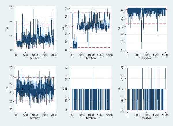
 h4            2000    0.398   0.193   0.0097    0.365 (  0.105,  0.897 )
 h5            2000    1.648   0.068   0.0024    1.647 (  1.512,  1.788 )
 s4            2000   28.418  10.649   1.5287   28.000 (  3.000, 45.000 )
 s5            2000   19.851   0.358   0.0120   20.000 ( 19.000, 20.000 )
 e4            2000   50.090   2.849   0.1463   51.000 ( 42.000, 52.000 )
 e5            2000   26.878   0.355   0.0118   27.000 ( 26.000, 27.000 )
----------------------------------------------------------------------------
The intercept, a, and the two regression coefficients, b and c, are reasonably close to my prior estimates, although perhaps the upward drift is a little larger than I was expecting.
Most of the epidemics are easy to detect but I have chosen to display results for one year without a clear epidemic and one with. The epidemic in year 4 is poorly defined. It has a low height and might start any time between week 3 and week 45. In contrast the epidemic in year 5 is much more clear cut. It raised the expected winter level by exp(1.6)≈5 times and almost certainly started in week 20 and finished in week 27.
Convergence is not a major problem although the estimated epidemic in year 4 does jump around and were we particularly interested in that year we would need a much longer run in order to capture its posterior. A more realistic solution might be to allow the model to have years in which there is no epidemic. Perhaps we will return to try that modification at a later date.
If we save the posterior mean estimates we can use them to plot a fitted curve
insheet using temp.csv , clear
mcmcstats *
forvalues i=1/39 {
local p`i’ = r(mn`i’)
}
use tempflu.dta, clear
gen eta = `p1′ + `p2’*time/1000 + `p3’*sin(0.060415*week)
forvalues i=1/12 {
local j = 3 + `I’
local h = `p`j”
local j = 15 + `i’
local S = `p`j”
local j = 27 + `i’
local E = `p`j”
replace eta = eta + `h’ if year == `i’ & week >= `S’ & week <= `E’
}
gen mu = exp(eta)
twoway (line chile time ) (line mu time, lcol(red) lpat(dash)) , leg(off)
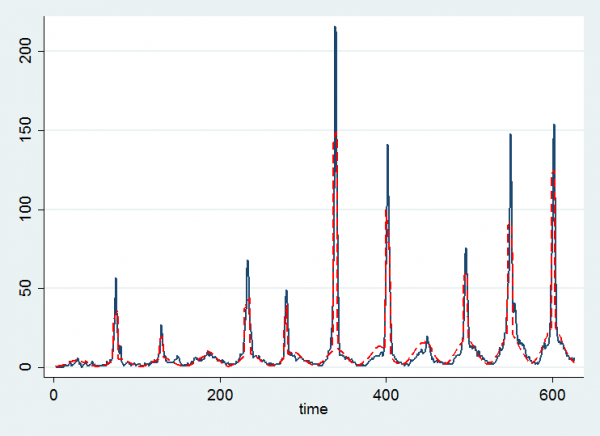
Here the black line represents the data and the red line is the fitted curve based on the posterior means. We seem to pick up the flu epidemics quite well and it is clear that the lack of an epidemic in year 4 and the strong epidemic in week 5 accord with the numerical results.
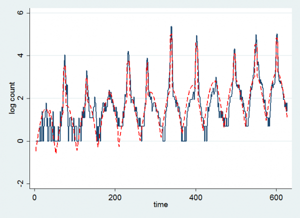
Since the model uses a log-link function we can see the fit better if we look at the log-count and the log of the fitted values.
The drift upwards is clearer although perhaps it was not linear over the whole range of the data. My overall impression is that the model has been relatively successful in capturing the trend.
There is much more to do but this is enough for one week.


 Subscribe to John's posts
Recent Comments