I am always on the lookout for interesting medical data sets that I can use for teaching and the other day, quite by accident, I came across “Google flu trends”. This is an internet project operated by Google that estimates the numbers of cases of influenza each week in 25 different countries. The records go back to the beginning of 2003.
The novel aspect of this project is that influenza is monitored by tracking online Google searches related to influenza. The number of searches has been calibrated against surveys of the number of medically diagnosed cases. You can find more information on Wikipedia.
There is a fascinating on-going debate in the media and on the internet about the ability of such search engine data to predict cases of influenza. What is most interesting is the emotion that this debate generates. People who are attracted by big data get enthusiastic about the project and play down its limitations, while people who equate big data with big brother stress the weakness in the flu estimates and overlook the potential. It is as though they are not really talking about Google flu trends but merely using the debate as a vehicle for justifying their wider prejudices.
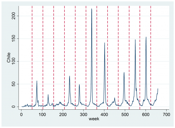
Anyway, I will just accept the data and see how we might model them to detect influenza epidemics. After all, even if the search based predictions are wrongly calibrated they might still rise when the true number of cases of flu rises, which could be enough to enable us to detect the start of an outbreak. As an example, here is the data for Chile.
The dashed vertical lines denote periods of 52 weeks. Remember that Chile is in the southern hemisphere so the winter influenza peak occurs around the middle of the year. Just looking at the plot one can see a small seasonal trend of the type that is most obvious in year 4 (around 200 weeks). Then on top of that there is usually an annual epidemic that causes a sharp spike of variable size and variable duration. For the purposes of monitoring influenza, we would like to analyse these data in real time and to decide as soon as possible when an epidemic is underway.
I will try to derive a Bayesian analysis of these data and in the process of developing and fitting such a model I will need to create a new sampler and integrate it into the general structure described in my book.
In my model the weekly counts will be thought of as being dependent on a latent variable that denotes whether or not an epidemic is in progress. We will define a variable Z that takes the value 0 when there is no current epidemic, and 1, when there is a current epidemic. Of course, Z is not observed but has to be inferred from the pattern of counts. Our aim is to detect as soon as possible when Z switches from 0 to 1.
It appears from the plot that it would be reasonable to start by assuming that there is exactly one flu epidemic every year and that the severity varies from the very minor (e.g. year 4) to the very extreme (year 7).
Each epidemic is characterised by the week that it starts, S, and the week that it ends, E. These parameters will take integer values and of course S must be less that E. It would be nice to be able to update estimates of S and E using a Metropolis-Hastings algorithm but the programs given in my book only work for parameters defined over a continuous range: mhsnorm is good for parameters defined over an infinite range (-∞,∞), mhslogn is good for (0,∞) and mhstrnc is good for (a,b), where a and b are finite. Our first job therefore is to design a new Metropolis-Hastings sampler that can deal with integer valued parameters.
Let’s suppose that θ is a parameter defined over the integers (1, 2, … , n) and and that we have a program that works out the log-posterior given θ. If the current value of the parameter is θ0, we need to make a proposal say θ1 and compare logpost(θ0) with logpost(θ1) to see if we accept a move to θ1 or reject it and stay at θ0.
We might propose a random move to any other integer in the range [1,n]. The disadvantage of completely random moves is that many of the proposed moves will take us to poorly supported values and such moves are very likely to be rejected. Lots of rejected moves will mean poor mixing.
An alternative strategy would be to propose a move to a neighbouring value, i.e. from θ0=12 to θ1=11 or 13. Such local moves are more likely to be accepted but the change is small so the algorithm will require lots of moves to cover the posterior and this might also be inefficient, especially early in the chain when we have not located the peak of the posterior.
On balance my gut feeling favours short moves to neighbouring points. So let’s assume that when θ0=12 we are equally likely to suggest a move up to 13 or a move down to 11. Similarly if θ0=11 we are equally likely to propose a move to 10 or 12. The key feature is Pr(propose 11 | θ0=12 ) = Pr(propose 12 | θ0=11 ). This is the characteristic that defines the special case known as a Metropolis algorithm in which the proposal probabilities cancel and we only need to worry about the comparative values of the log-posterior.
There is a small problem at the end points of the range. Consider the case when θ0=1, the move to θ1=0 is not allowed because the range is [1,n]. We can cope with this, either by modifying the rule for making proposals, or by making the log-posterior at θ1=0 so small that the move is never accepted. The latter is easier to program.
The program for the new sampler will follow the same pattern as mhsnorm. So let’s look at that program and see what needs to be changed. I have highlighted the few places that need our attention in green.
program mhsnorm, rclass
syntax anything [fweight] [if] [in], SD(string) [ LOGP(real 1e20) DEBUG ]
tokenize “`anything'”
local logpost “`1′”
local b “`2′”
local ipar = `3′
tempname logl newlogl
if “`debug'” == “” local qui “qui”
local oldvalue = `b'[1,`ipar’]
scalar `logl’ = .
if `logp’ < 1e19 scalar `logl’ = `logp’
if `logl’ == . {
`qui’ `logpost’ `logl’ `b’ `ipar’ [`weight’`exp’] `if’ `in’
if `logl’ == . {
di as err “mhsnorm: cannot calculate log-posterior for parameter `ipar'”
matrix list `b’
exit(1400)
}
}
matrix `b'[1,`ipar’] = `oldvalue’ + `sd’*rnormal()
scalar `newlogl’ = .
`qui’ `logpost’ `newlogl’ `b’ `ipar’ [`weight’`exp’] `if’ `in’
if `newlogl’ == . {
di as err “mhsnorm: cannot calculate log-posterior for parameter `ipar'”
matrix list `b’
exit(1400)
}
if log(uniform()) < (`newlogl’-`logl’) local accept = 1
else {
local accept = 0
matrix `b'[1,`ipar’] = `oldvalue’
scalar `newlogl’ = `logl’
}
return scalar accept = `accept’
return scalar logp = `newlogl’
end
Most of the program is involved in housekeeping and error checking so the changes are minimal. First, since I am going to call the new sampler mhsint, we need to change all references to mhsnorm into mhsint, then we need to drop the redundant SD option and finally we change the line that makes the new proposal from
matrix `b'[1,`ipar’] = `oldvalue’ + `sd’*rnormal()
to
matrix `b'[1,`ipar’] = `oldvalue’ + 1 – 2*(runiform()<0.5)
This ensures that the proposal has an equal chance of being 1 more or 1 less that the previous value.
Let’s design a simple test to show how mhsint can be used with mcmcrun in just the same way as the other samplers mentioned in my book. I will suppose that a variable can take the values 1 or 2 or 3 with posterior probabilities 0.2, 0.3 and 0.5. Here is a program for calculating the log-posterior. If we move outside the range [1,3] then the log-posterior is set to a very low number so as to effectively block the move.
program logpost
args lnf b
local k = `b'[1,1]
if `k’ == 1 scalar `lnf’ = log(0.2)
else if `k’ == 2 scalar `lnf’ = log(0.3)
else if `k’ == 3 scalar `lnf’ = log(0.5)
else scalar `lnf’ = -999.9
end
I’ll start the run with the variable (that I’m calling k) set to 2. This I use mcmcrun to create a short burnin and then 500 samples.
matrix b = (2)
mcmcrun logpost b using temp.csv, replace ///
param(k) burn(50) update(500) samp( mhsint )
insheet using temp.csv , clear
tabulate k
          k |     Freq.     Percent       Cum.
------------+-----------------------------------
          1 |       102       20.40       20.40
          2 |       145       29.00       49.40
          3 |       253       50.60      100.00
------------+-----------------------------------
      Total |       500     100.00
Clearly the chain has settled to the correct proportions.
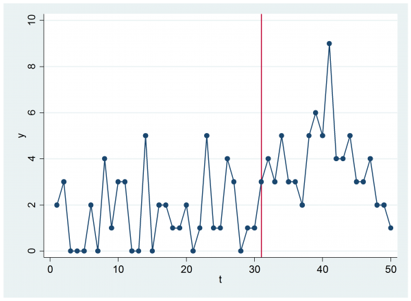
Next let’s design a test that is closer to the flu problem. Suppose that we generate at sequence of 50 values, i.e. the flu counts for each week over most of a year. At the start of the year the counts will be Poisson with a mean of 2 but at some random point between 10 and 40 weeks they will switch to a Poisson with a mean of 4.
clear
set seed 626169
set obs 50
local start = int(10+runiform()*31)
gen t = _n
gen mu = 2 + 2*(t >= `start’)
gen y = rpoisson(mu)
scatter y t, c(l) xline(`start’)
In this simulation the switching point is at 31. What we need to do is to estimate the time of the switch, which I’ll again call k, from the 50 counts.
Here is a program that calculates the log-posterior. If we step outside the range [10,40] then the move is blocked by setting a very small log-posterior, otherwise we calculate a standard Poisson log-likelihood with known means 2 or 4 and a switch at the current k, which is stored as the first element of our parameter vector, b.
program logpost
args lnf b
if `b'[1,1] < 10 | `b'[1,1] > 40 scalar `lnf’ = -9999.9
else {
tempvar mu lnL
gen `mu’ = 2
qui replace `mu’ = 4 if _n >= `b'[1,1]
gen `lnL’ = y*log(`mu’) – `mu’
qui su `lnL’
scalar `lnf’ = r(sum)
}
end
We can run the analysis much as before
matrix b = (25)
mcmcrun logpost b using temp.csv, replace ///
param(k) burn(50) update(500) samp( mhsint )
insheet using temp.csv , clear
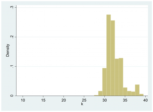
histogram k , start(9.5) width(1) xlabel(10(5)40)
The estimated log-posterior does indeed peak at 31 but given the nature of the data that we saw in the time series plot it is not surprising that the switch looks more likely to have come later in the sequence rather than earlier.
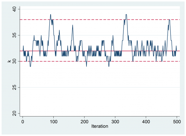
If we inspect the trace plot of the chain then we can see that we only made steps of size one but, despite this, the mixing looks reasonable.
It would be a simple matter to change from steps of size 1 to steps of size 1 or 2 or steps of size 1 or 2 or 3. We just need to change the line of code that creates the random proposal.
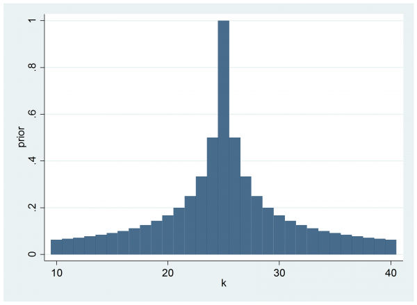
As it stands, the program logpost does not include a prior on k, so the implicit assumption is that prior to seeing the data we thought that all switching points in the range [10,40] were equally likely. As it happens, this accords with the way that the data were generated but had the data been real counts of flu in a small population, we might well have had prior belief about when the switch would occur. For example, we might believe that 25 is the most likely switching point and that the prior probability is proportional to 1/(1+abs(k-25))
clear
range k 10 40 31
gen prior = 1/(1+abs(k-25))
twoway bar prior k
We can incorporate this prior into the calculation of the log-posterior
program logpost
args lnf b
if `b'[1,1] < 10 | `b'[1,1] > 40 scalar `lnf’ = -9999.9
else {
tempvar mu lnL
gen `mu’ = 2
qui replace `mu’ = 4 if _n >= `b'[1,1]
gen `lnL’ = y*log(`mu’) – `mu’
qui su `lnL’
scalar `lnf’ = r(sum) – log(1+abs(`b'[1,1]-25))
}
end
and the posterior is pulled slightly to the left.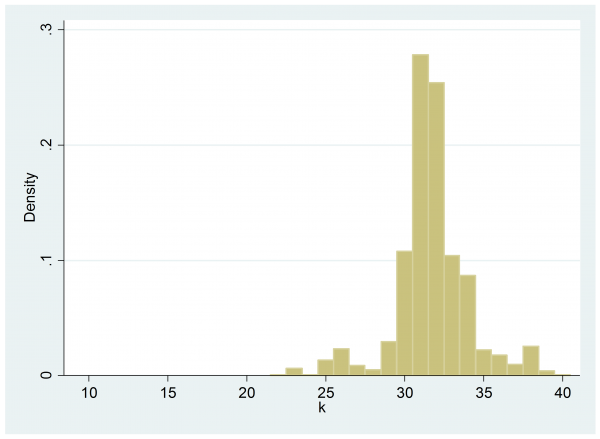
Next time I will use the new sampler to help me build a model for the flu data.


 Subscribe to John's posts
Recent Comments