Every few weeks I try to find an hour or so to browse through the latest issues of the main statistics journals. This gives me the opportunity to read papers on topics that I know relatively little about; it is my way of keeping up to date with new developments beyond my day to day work on genetic epidemiology. Of course, it is only possible to read a handful of these papers and one of the ways that I select those that I will read is to follow a few well-known authors who are good at explaining their work to non-specialists.
One of the authors that I look out for is Bradley Efron and a few weeks ago I came across one of his latest papers. It has a Bayesian theme, so I thought that it would be worth mentioning in this blog. The reference is,
Efron B
Frequentist accuracy of Bayesian estimates
Journal of the Royal Statistical Society, Series B 2015;77:617-646
The paper addresses the question, how do you assess the accuracy of a Bayesian parameter estimate when you use a convenience or reference prior?
My short answer to this question is that you should not use a convenience or reference prior. In my opinion you should always think about your priors and if you know little about the parameters then choose a prior that is realistically vague, rather than relying on a standard zero centred normal prior with a huge variance, or a Jeffrey’s prior, or whatever.
None the less there are plenty of people who advocate objective Bayesian methods (Berger 2006 is probably best reference) and since I do not accept the objective Bayesian argument, I feel compelled to try to be fair to them.
Objective Bayes comes it many forms and there is an honourable tradition of trying to find priors that produce posterior distributions with good theoretical properties, often good frequentist properties. Unfortunately, this has proved very difficult and in practice what passes for objective Bayes may just be the adhoc use of supposedly noninformative priors. These priors cannot be said to reflect anyone’s real prior opinion, so the question for people who use them is, what do your results mean?
The usual Bayesian interpretation of a 95% credible interval is that you believe that there is a 0.95 probability that the parameter lies in the interval. However, the calculation of the interval is conditional on both the model and the prior. If you do not believe in the prior, how can you make statements of belief based on the posterior?
Adhoc objective Bayesians can of course say that their analysis applies to a hypothetical individual who holds these reference beliefs, but often the objective priors are so extreme that it is hard to imagine any real person with that degree of ignorance.
Alternatively, they can appeal to a type of robustness and say that their prior gives results very similar to other noninformative priors and so they can claim to have a standard analysis that will apply to anyone who does not have strong prior knowledge. This would be fine if it were not for the fact that robustness to the choice of prior is problem specific. In complex models it can be that seemingly noninformative priors do influence the results. So to justify the robustness, the researchers ought really to consider a wide range of noninformative priors.
Efron investigated a frequentist solution to assessing the accuracy of a Bayesian analysis. It would apply to any analysis, whether or not an objective prior was used, but its main application is likely to be in objective Bayesian analysis when the justification for the prior lies in the good frequentist properties of the results that it produces.
I am going to use a slightly different notation to Efron, so be warned.
The idea is to estimate some parameter that interests us using its posterior mean, let’s call it β(x) to emphasise that it is an estimate based on the real data, x. As part of the Bayesian analysis we will have specified a data generating model f(x|θ), where in my notation θ is the full set of parameters, and a prior, π(θ), that might or might not reflect someone’s real beliefs. The Bayesian analysis also provides the posterior mean estimates θ(x).
So we could use the data generating model f(x*|θ(x)) to simulate a new data set x*. In which case, we could analyse x* to obtain the posterior mean estimate of the important parameter, β(x*). Given enough computing power we could create thousands of simulated datasets and thousands of Bayesian estimates of β.
A histogram of the β’s would be an approximation to the sampling distribution for β from which we could obtain the frequentist standard deviation, which in this context is usually called the standard error. Provided that the sampling distribution is shaped roughly like a normal distribution, the standard error will lead us to an approximate 95% confidence interval.
The important point is that this 95% confidence interval will have the usual frequentist interpretation, i.e. 95% of such intervals would include the true β and this interpretation will not depend on believing in the prior, π(θ).
As you might imagine this process would be computationally very demanding, so Efron provides a short cut in the form of an approximation to the standard error. He shows that the variance of the sampling distribution is approximately,
Cov(β,α)’V(µ |θ) Cov(β,α)
and the standard error is the square root of this variance.
In this formula, V(µ|θ) is the posterior covariance matrix of µ, the predicted values of x, and α relates small changes in the data to the standard deviation via the log of the density; it is the vector of derivatives,
d log f(x|θ)/dxi
This is not a trivial calculation. If there are n observations and one β, the matrix V will nxn and Cov(β,α) will be nx1.
As you would expect in a paper by Bradley Efron, he goes on to consider using the ideas of bootstrapping to improve the confidence interval and also discusses some simplifications that result when the data generating model is a member of the exponential family.
Let’s see how we might find the approximate standard error in Stata.
In the article Efron presents data from an experiment in which mouse nuclei were introduced into colonies of human cells. Batches of colonies were infused with one of five proportions of mouse nuclei and left for between 1 and 5 days. Each colony was eventually classified as ‘thriving’ or not and the data consist of the number thriving out of the number of colonies.
| Day D=1 | D=2 | D=3 | D=4 | D=5 | |
| Proportion I=1 | 5/31 | 3/28 | 20/45 | 24/47 | 29/35 |
| I=2 | 15/77 | 36/78 | 43/71 | 56/71 | 66/74 |
| I=3 | 48/126 | 68/116 | 145/171 | 98/119 | 114/129 |
| I=4 | 29/92 | 35/52 | 57/85 | 38/50 | 72/77 |
| I=5 | 11/53 | 20/52 | 20/48 | 40/55 | 56/61 |
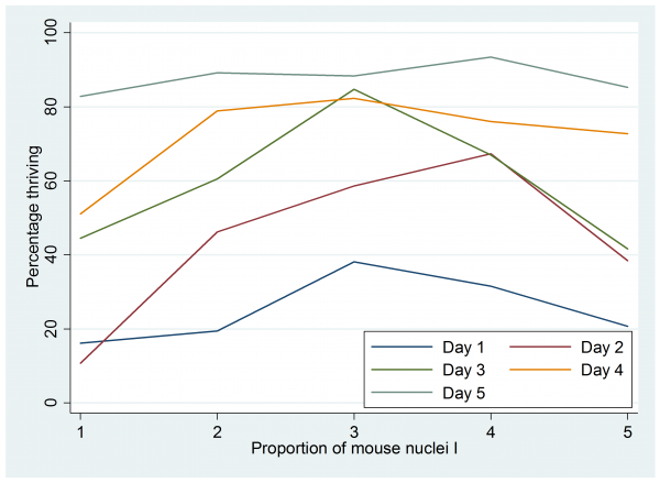
I entered these data into Stata as 4 columns of 25 rows and I called the columns, I, D, x and n. Then I saved the data in a file call cell.dta and plotted the percentages that thrived.
gen p=100*x/n
twoway (line p I if D==1) (line p I if D==2) ///
(line p I if D==3) (line p I if D==4) (line p I if D==5) , legend(ring(0) pos(5) ///
label(1 “Day 1”) label(2 “Day 2”) label(3 “Day 3”) label(4 “Day 4”) label(5 “Day 5”) ) ///
xtitle(“Proprtion I”) ytitle(“Percentage thriving”)
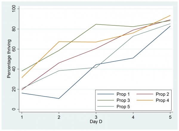
Perhaps it would be better to plot the logit of the proportion thriving rather than the percentage but that plot looks almost identical and the percentage scale is easier to understand. There seems to be some justification for including a quadratic term in the proportion I, but a similar plot against day shows no evidence of a quadratic term.
Despite this Efron uses a Binomial model with probability pjk where
logit(pjk) = θ0 + θ1I + θ2I2 + θ3D + θ4D2
j denoted proportion 1 to 5 and k denotes day
For illustration I will adopt the same structure.
Efron supposes that our interest is in β = Average(pj5)/Average(pj1), that is the ratio of the average probability of thriving on day 5 compared with the average probability on day 1.
Now we will do what I consider to be the wrong thing and use a prior that I do not believe in. Let’s choose θi ~ N(0,sd=100).
This is a simple model to fit in Stata. The log posterior can be calculated by,
program logpost
args lnf b
local theta0 = `b'[1,1]
local theta1 = `b'[1,2]
local theta2 = `b'[1,3]
local theta3 = `b'[1,4]
local theta4 = `b'[1,5]
tempvar eta lnL
gen `eta’ = `theta0′ + `theta1’*I + `theta2’*I*I + `theta3’*D + `theta4’*D*D
gen `lnL’ = x*`eta’ – n*log(1+exp(`eta’))
qui su `lnL’
scalar `lnf’ = r(sum) – (`theta0’*`theta0’+`theta1’*`theta1’+ ///
`theta2’*`theta2’+`theta3’*`theta3’+`theta4’*`theta4′)/20000
end
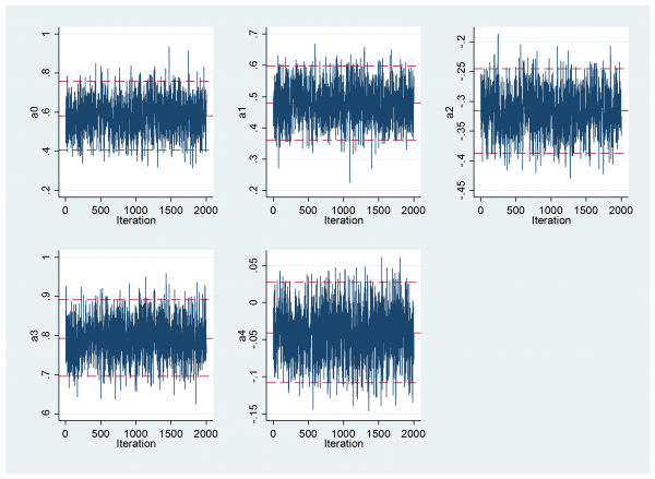
and the model can be fitted using mcmcrun. Notice the use of centring of I and D; this gives an equivalent model but the reparameterization reduces the correlation between the parameters and so improves the mixing.
use cell.dta, clear
replace I = I – 2.5
replace D = D – 2.5
matrix b = (0.0, 0.0, 0.0, 0.0, 0.0)
matrix s = (0.05, 0.05, 0.05, 0.05, 0.05)
mcmcrun logpost b using temp.csv, replace samplers( 5(mhsnorm , sd(s) ) ) adapt ///
param(theta0 theta1 theta2 theta3 theta4) burn(5000) update(20000) thin(10)
matrix list s
insheet using temp.csv, clear
mcmcstats_v2 theta* , newey(50) corr
mcmctrace theta*
----------------------------------------------------------------------------
Parameter         n     mean       sd      sem   median         95% CrI
----------------------------------------------------------------------------
 theta0        2000    0.583    0.090   0.0027    0.582 (   0.407,   0.759 )
 theta1        2000    0.478    0.060   0.0020    0.478 (   0.362,   0.597 )
 theta2        2000   -0.316    0.036   0.0012   -0.316 (  -0.388,  -0.245 )
 theta3        2000    0.792    0.049   0.0012    0.793 (   0.696,   0.891 )
 theta4        2000   -0.041    0.034   0.0009   -0.041 (  -0.108,   0.028 )
----------------------------------------------------------------------------
We can use these results to calculate the ratio beta. I first read the data and saved the n’s as locals then I re-read the mcmc results, and calculated the probabilities from the logit model and the expected numbers that thrived. Beta is just a function of those probabilities.
use cell.dta,clear
forvalues i=1/25 {
local n`i’ = n[`i’]
}
insheet using temp.csv, clear
local k = 0
forvalues i=1/5 {
forvalues d=1/5 {
local ++k
gen eta`k’ = theta0+theta1*(`i’-2.5)+theta2*(`i’-2.5)*(`i’-2.5)+ ///
theta3*(`d’-2.5)+theta4*(`d’-2.5)*(`d’-2.5)
gen p`k’ = invlogit(eta`k’)
gen mu`k’ = `n`k”*p`k’
}
}
gen beta = (p5+p10+p15+p20+p25)/(p1+p6+p11+p16+p21)
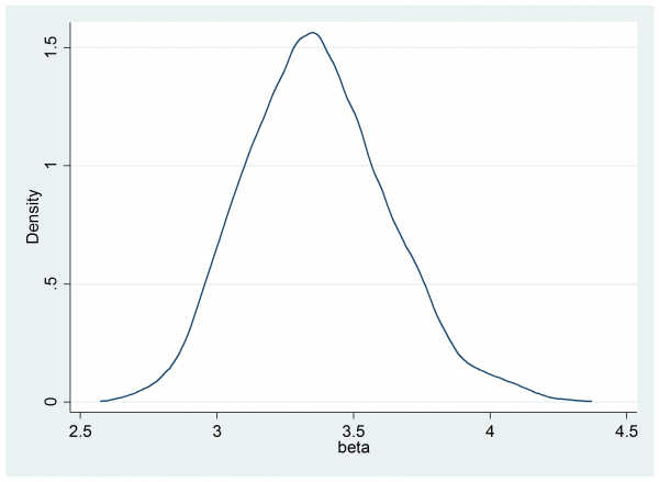
mcmcstats_v2 beta, newey(50)
mcmcdensity beta
----------------------------------------------------------------------------
Parameter         n     mean       sd      sem   median         95% CrI
----------------------------------------------------------------------------
 beta          2000    3.367    0.261   0.0057    3.356 (   2.896,   3.938 )
----------------------------------------------------------------------------
So if we had believed in the prior we would be able to say that now we believe with probability 0.95 that beta is between 2.90 and 3.94. But we do not really believe in the prior so we need some other way of expressing the results.
In order to study the frequentist properties of our analysis, we need to calculate the covariance matrix V and the vector of 25 derivatives with respect to each of the x’s.
For the binomial model the log-likelihood has the form
Sumj,k {xjklog(pjk) + (njk-xjk)log(1-pjk) }
A little algebra shows that in terms of θ this becomes
Sumj,k {xjk[θ0 + θ1j + θ2j2 + θ3k + θ4k2] – njklog(1+exp[θ0 + θ1j + θ2j2 + θ3k + θ4k2]) }
If we differentiate with respect to xjk we get
αjk = θ0 + θ1j + θ2j2 + θ3k + θ4k2
Now we are in a position to find V and the covariances and to combine them to get the approximate standard error.
matrix accum V = mu*, nocon dev
matrix V = V/2000
matrix COV = J(1,25,0)
forvalues i=1/25 {
qui corr beta eta`i’ , cov
matrix COV[1,`i’] = r(cov_12)
}
matrix VAR = COV*V*COV’
di sqrt(VAR[1,1])
The answer is that the approximate standard error is 0.252.
You will have noticed that this standard error is very close to the standard deviation of the posterior, which was 0.261.
The slightly disappointing thing about this method is that, in most cases, the frequentist standard error will turn out to be almost identical to the posterior standard deviation. So the slightly ignorant approach of treating the credible interval as being interchangeable with a confidence interval will often work.
None the less it seems to me that deriving the frequentist properties of a Bayesian solution offers the only practical hope for objective Bayesian analysis. Of course, it is simpler and better to use priors that you actually believe in.


 Subscribe to John's posts
Recent Comments