A rather long posting this week for which I apologise. I would have split this posting over two weeks but I am about to go on my summer holiday and I wanted to avoid a long gap between the two halves.
I have spent the last few weeks discussing how Stan can be called from Stata and now the time has come to test the process with a realistic problem. To create a comparison, I thought that I would take a problem that is challenging for OpenBUGS and see whether Stan offers any advantages. In the spirit of this blog, the question ought to be,
is it as easy to run Stan from Stata, as it is to run OpenBUGS from Stata?
but the answer to that question is clearly, yes, so inevitably we will get drawn into the issue,
is Stan as good as OpenBUGS?
For my test problem I have chosen a network meta-analysis as described in,
White I.R., Barrett J.K., Jackson D, Higgins J.P.T.
Consistency and inconsistency in network meta-analysis: model estimation using multivariate meta-regression
Research Synthesis Methods 2012;3:111-125
In that paper the authors present the data for a worked example and give the WinBUGS code for fitting their model; so much of my work is done for me. What is more, their analysis was performed with three chains, each with a burn-in of 30,000 and a run length of 150,000 so the model is clearly challenging enough to make a good test.
I’ve blogged about network meta-analysis before here and here. I have to admit to having some doubts about its usefulness but I was impressed that the paper by White et al. addresses one of my main concerns, how do we detect when a network meta-analysis is inconsistent?
The example used in the paper is a meta-analysis of 28 trials of drug treatments given to people who had had a heart attack. The outcome was the number of deaths in the first month after treatment. 8 different drugs were compared in the trials but the designs varied; for instance, some compared streptokinase with alteplase, some compared streptokinase with urokinase, yet others compared alteplase with urokinase and so on.
Well, if streptokinase is better than alteplase by one unit on some outcome scale and alteplase is better than urokinase by one unit on the same scale, then streptokinase ought to be better than urokinase by two units. If this is so, then the data are said to be consistent. It is possible however that the streptokinase-urokinase trials were different in some systematic way, perhaps they were conducted more recently or they all come from the USA. If they do differ systematically then the directly measured effect may not be consistent with the indirectly implied effect. White et al. refer to the set of treatments compared in a study as the ‘design’ and handle inconsistency by treating it as an interaction between the treatment effect and the design.
There is much more to the model that they propose but I do not think that it is necessary for us to understand all of the details as our primary interest is in seeing if Stan can handle it.
Let’s first fit the model with design by treatment interaction using OpenBUGS and the code provided in White et al. I have removed a few lines from White et al.’s program that calculate derived quantities that are not essential for the estimation. The data, taken from Table 1 of the paper, are in a file called thrombolytic.dta that is available from my webpage along with all of the Stata code .
Here is the full Stata program.
use “thrombolytic.dta”, clear
* Number of treatments in each study
sort study
by study: egen nt = count(trt>0)
* offsets – row numbers for start of each study or design
sort design study trt
gen os = _n*(study != study[_n-1])
gen os_design = _n*(design != design[_n-1])
by design: egen b = min(trt)
replace os = 59 in 58
* Write data to file
wbslist (vect study design trt b r n, format(%5.0f) name(study d t b r n) ) ///
(vect os if os != 0 , format(%5.0f) name(offset) ) ///
(vect os_design nt if os_design != 0 , format(%5.0f) name(offset.design num.ests) ) ///
(zero=c(7{0})) (A=58, S=28, T=8, D=13) using data.txt, replace
* Prepare three sets of starting values for 3 chains
matrix RE = J(28,8,0)
forvalues i=1/28 {
matrix RE[`i’,1] = .
}
wbslist (matrix RE , format(%5.0f) ) ( mu=c(28{-1}) ) ( tau=0.2) ///
using init1.txt, replace
wbslist (matrix RE , format(%5.0f) ) ( mu=c(28{-2}) ) ( tau=1) ///
using init2.txt, replace
wbslist (matrix RE , format(%5.0f) ) ( mu=c(28{-1.5}) ) ( tau=0.5) ///
using init3.txt, replace
* Write the model
wbsmodel thrombo_bayes.do model.txt
/*
model {
for(i in 1:S) {
eff.study[i, b[offset[i]], b[offset[i]]] <- 0
for(k in (offset[i] + 1):(offset[i + 1]-1)) {
eff.study[i,t[k],b[k]] <- eff.des[d[k],t[k]] + RE[i,t[k]] – RE[i,b[k]]
}
}
# Random effects for heterogeneity
for(i in 1:S) {
RE[i,1] <- 0
RE[i,2:T] ~ dmnorm(zero[], Prec[,])
}
# Prec is the inverse of the structured heterogeneity matrix
for(i in 1:(T-1)) {
for(j in 1:(T-1)){
Prec[i,j] <- 2*(equals(i,j)-1/T)/(tau*tau)
}
}
for(i in 1:A) {
logit(p[i]) <- mu[study[i]] + eff.study[study[i],t[i],b[i]]
r[i] ~ dbin(p[i],n[i])
}
# Priors
for(i in 1:S) {
mu[i] ~ dnorm(0,0.01)
}
tau ~ dunif(0,2)
for(i in 1:D) {
for(k in (offset.design[i] + 1):(offset.design[i] + num.ests[i])) {
eff.des[i,t[k]] ~ dnorm(0,0.01)
}
}
}
*/
* Prepare the script
wbsscript using script.txt , replace openbugs ///
model(model.txt) data(data.txt) init(init1.txt+init2.txt+init3.txt) ///
set(tau eff.des RE mu) burn(30000) update(150000) thin(20) ///
log(openlog.txt) coda(thromb)
* Run the analysis
wbsrun using script.txt , openbugs
* check the log file
type openlog.txt
* read results and store
wbscoda using thromb , openbugs clear chains(1 2 3)
save thrombmcmc123.dta, replace
* calculate the interaction terms
gen w1 = eff_des_3_3 – eff_des_2_3 // wAC3
gen w2 = eff_des_4_4 – eff_des_1_4 // wAD4
gen w3 = eff_des_9_6 – eff_des_5_6 + eff_des_1_2 // wAF9
gen w4 = eff_des_10_7 – eff_des_6_7 + eff_des_1_2 // wAG10
gen w5 = eff_des_12_7 – eff_des_6_7 + eff_des_2_3 // wAG12
gen w6 = eff_des_7_8 – eff_des_2_8 // wAH7
gen w7 = eff_des_11_8 – eff_des_2_8 + eff_des_1_2 // wAH11
gen w8 = eff_des_13_8 – eff_des_2_8 + eff_des_2_3 // wAH13
gen dAE = eff_des_8_5 + eff_des_1_2
* various convergence checks
mcmctrace w1 w3 w5 w7 , gopt( xline(7500) xline(15000) yscale(range(-4 6)) ///
ylabel(-4(2)6) xscale(range(0 22500)) xlabel(0(5000)20000) )
mcmcstats_v2 w* , newey(200)
gen w7_1 = w7 if chain == 1
gen w7_2 = w7 if chain == 2
gen w7_3 = w7 if chain == 3
mcmcac w7_1 w7_2 w7_3 , gopt(yscale(range(0 0.5)) ylabel(0(0.2)0.4) ) acopt(lag(50))
Here we have 3 chains each with a burnin of 30,000 and a run length of 150,000 which makes 540,000 iterations. On my laptop, OpenBUGS took about 1s for 1000 updates so that the entire run took about 9 minutes. Here are the results for the interaction terms based on the combined chains. The results are very similar to those given in the paper and the only interaction that is clearly non-zero is w7
----------------------------------------------------------------------------
Parameter         n     mean       sd     sem   median         95% CrI
----------------------------------------------------------------------------
w1           22500   -0.165   0.366   0.0111   -0.103 ( -1.038,   0.452 )
w2           22500    0.479   0.808   0.0085    0.470 ( -1.101,   2.092 )
w3           22500   -0.193   0.504   0.0103   -0.158 ( -1.300,   0.775 )
w4           22500    0.387   0.791   0.0091    0.374 ( -1.136,   1.992 )
w5           22500    0.034   0.762   0.0107    0.034 ( -1.490,   1.545 )
w6           22500   -0.049   0.468   0.0095   -0.050 ( -0.991,   0.896 )
w7           22500    1.263   0.634   0.0138    1.247 (  0.049,   2.561 )
w8           22500   -0.321   0.505   0.0064   -0.319 ( -1.330,   0.674 )
----------------------------------------------------------------------------
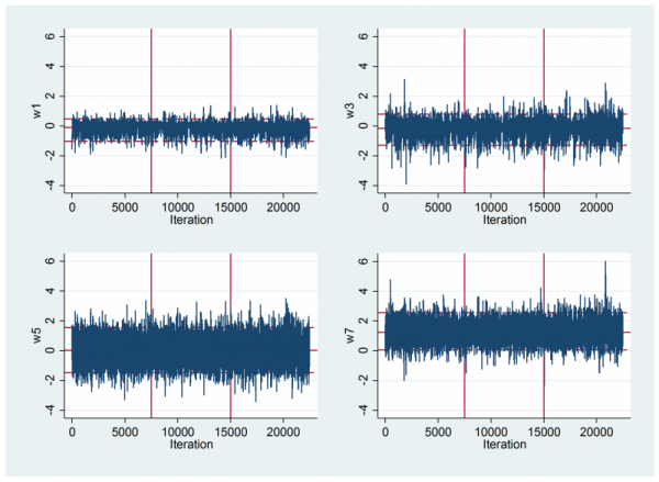
To inspect the mixing I looked at some trace plots. As usual they are not particularly informative. The vertical lines separate the three chains.
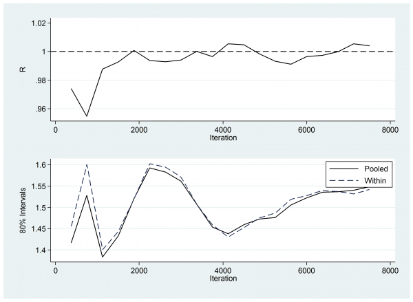
So next I checked the Brooks-Gelman-Rubin plots. Here is the plot for w7.
This plot compares the within chain variability to the variability of the pooled chains, R being the ratio of the two. Ideally R should be 1.0. Perhaps the first 1,000 thinned iterations have not quite settled, which would argue for a slightly longer burnin or better starting values.
To check this I ran a version of the Geweke test as implemented in mcmcgeweke. This compares w7 as calculated from the first 10% of each chain with the value from the final 50%. Not only is there evidence of drift, but the three estimates from the second halves of the chains are still subject to quite a lot of sampling error.
| First 10% | Last 50% | ||||
| Mean | St Error | Mean | St Error | p-value | |
| Chain 1 | 1.342 | 0.051 | 1.249 | 0.014 | 0.080 |
| Chain 2 | 1.149 | 0.028 | 1.267 | 0.014 | 0.0001 |
| Chain 3 | 1.159 | 0.037 | 1.322 | 0.022 | 0.0002 |
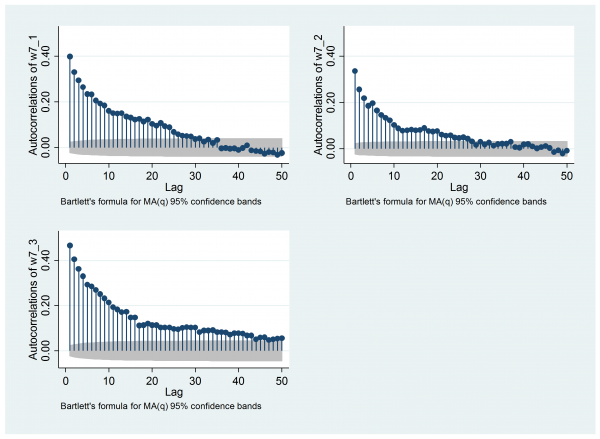
The reason that such a long chain is required is the strong autocorrelation. For me the autocorrelation plot is key. Remember that the stored values have already been thinned by 20, yet when we look at the autocorrelations for the three chains using mcmcac there is still noticeable correlation up to a lag of about 30 (that is, about 600 of the original iterations).
There are convergence issues that remain with the OpenBUGS analysis but it is time to try the same model in Stan. I’ll start by presenting a basic Stata program that performs the analysis and then I’ll discuss the changes in the code that are needed when we switch from OpenBUGS to Stan.
Here is the Stata program
use “thrombolytic.dta”, clear
* Number of treatments in each study
sort study
by study: egen nt = count(trt>0)
* offsets – row numbers for start of each study or design
sort design study trt
gen os = _n*(study != study[_n-1])
gen os_design = _n*(design != design[_n-1])
by design: egen b = min(trt)
replace os = 59 in 58
*——————————————————–
* Write the data file: jags & Stan use the same format
*——————————————————–
wbslist_v2 (vect study design trt b r n, format(%5.0f) name(study d t b r n) ) ///
(vect os if os != 0 , format(%5.0f) name(offset) ) ///
(vect os_design nt if os_design != 0 , format(%5.0f) name(offset_design num_ests) ) ///
(zero <- c(7{0.0})) (A <-58 _n S <- 28 _n T <- 8 _n D <- 13) ///
using thromData.txt, replace jags
*—————————————
* Write the model file
*—————————————
wbsmodel thrombo_stan.do thromModel.stan
/*
data {
int A; int S; int T; int D;
int study[A]; int d[A]; int t[A]; int b[A]; int r[A]; int n[A];
int offset[29]; int offset_design[13]; int num_ests[13];
vector[7] zero;
}
parameters {
real<lower=0.0,upper=2.0> tau;
real eff_des[A,A];
vector[7] RE[S];
real mu[S];
}
transformed parameters {
matrix[7,7] Prec;
real eff_study[S,A,A];
# Prec is the inverse of the structured heterogeneity matrix
for(i in 1:7) {
Prec[i,i] <- 1.75/(tau*tau);
for(j in 1:7){
if( i != j ) Prec[i,j] <- -0.25/(tau*tau);
}
}
for(i in 1:S) {
eff_study[i, b[offset[i]], b[offset[i]]] <- 0;
for(k in (offset[i] + 1):(offset[i + 1]-1)) {
if( t[k] == 1 ) {
if( b[k] == 1 ) eff_study[i,t[k],b[k]] <- eff_des[d[k],t[k]];
else eff_study[i,t[k],b[k]] <- eff_des[d[k],t[k]] – RE[i][b[k]-1];
}
else {
if( b[k] == 1 ) eff_study[i,t[k],b[k]] <- eff_des[d[k],t[k]] + RE[i][t[k]-1];
else eff_study[i,t[k],b[k]] <- eff_des[d[k],t[k]] + RE[i][t[k]-1] – RE[i][b[k]-1];
}
}
}
}
model {
# Random effects for heterogeneity
for(i in 1:S) {
RE[i] ~ multi_normal_prec(zero, Prec);
}
for(i in 1:A) {
r[i] ~ binomial_logit(n[i],mu[study[i]] + eff_study[study[i],t[i],b[i]]);
}
# Priors
for(i in 1:S) {
mu[i] ~ normal(0.0,10.0);
}
tau ~ uniform(0.0,2.0);
for(i in 1:D) {
for(k in (offset_design[i] + 1):(offset_design[i] + num_ests[i])) {
eff_des[i,t[k]] ~ normal(0.0,10.0);
}
}
}
*/
*—————————————
* Prepare a Stan batch file
*—————————————
wbsscript_v3 using throm.bat , replace ///
model(thromModel.stan) data(thromData.txt) ///
updates(3000) burnin(500) coda(outthromprec) stan
*—————————————
* Run the batch file
*—————————————
wbsrun_v3 using throm.bat , stan
type log.txt
*—————————————
* read the results into Stata
*—————————————
wbscoda_v3 using outthromprec.csv , stan clear
The Stata code for preparing the data file is almost unchanged. Stan uses the same data file format as JAGS, so we merely set the jags option to wbslist_v2. Note though that when we do not use a keyword, wbslist_v2 writes our text directly to the file and in the JAGS/Stan format each item must be placed on a newline, so _n replaces the comma of OpenBUGS as our separator.
We do not need initial values as Stan is designed to set them internally.
After specifying the model we create a script file with wbsscript_v3 much as with OpenBUGS except that we set the stan option. Remember that the file that is created is actually a batch file and not a script file because Stan works by compiling the code in the model file and turning it into an executable program that is run via the Windows operating system.
The results are written to a comma delimited file that could be read by Excel. However, the file contains a header of summary information about the run so we need to use wbscoda_v3 to extract the simulations and to read them into Stata.
This leaves us with the Stan model file. Of course there are many ways of writing any piece of computer code and my experience of Stan is rather limited so my code may not be the most efficient, but at least it works.
The first block defines the data and sets up space for the information that will be read from the data file. Remember that Stan does not see the data until after the program has been compiled so it needs to be told the sizes of the variables. The next block defines the parameters, i.e. everything for which you give a prior. Stan will choose random starting values for these parameters. Next come the transformed parameters. These are quantities that can be calculated from the basic parameters. For instance, the precision matrix, Prec, can be calculated from tau. Stan will obtain the starting values for the transformed parameters by deriving them from the starting values for the basic parameters.
When the elements of Prec are calculated from tau, the OpenBUGS code used the equals() function, while in Stan I code the test explicitly using “== “
You will notice some other differences in the code. In OpenBUGS we had a matrix of parameters RE in which the first column was fixed at zero and the other columns were estimated. Use of fixed and estimated values in the same structure is not allowed in Stan so I formed a parameter matrix RE with one less column and treated references to column 1 as a special case in the subsequent code. In fact I have not defined RE to be a matrix at all, but rather I have created a set of vectors corresponding to the different columns. This is somewhat more natural since each vector(column) is drawn separately from a multivariate normal distribution.
Finally, notice that the distributions have different names in Stan and there are many variations on each distribution. So a multivariate normal, multi_normal(), is used if you know the mean and covariance matrix and multi_normal_prec() is used if you know the mean and precision matrix. binomial() is used when we know n and p, but binomial_logit() is used when we know n and logit(p).
The Stan syntax takes a little getting used to if you are a long-standing BUGS user, but in truth it is closer to a standard programming language and much more flexible than WinBUGS or OpenBUGS.
Anyway the code runs, but don’t start it if you are in a hurry. It is incredibly slow! 3000 updates and a 500 burnin took about 1.5 hours.
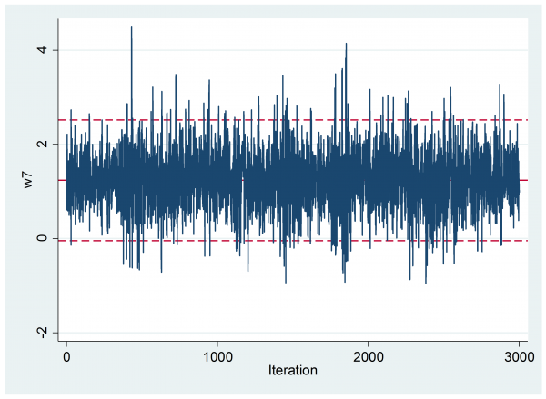
Although Stan is very slow, the estimates that it produces are of very high quality. The 3,000 updates have a similar sem to that given by 450,000 OpenBUGS updates.
—————————————————————————-
Parameter n mean sd sem median 95% CrI
—————————————————————————-
w7 3000 1.249 0.646 0.0141 1.239 ( -0.048, 2.515 )
—————————————————————————-
What is more there is no indication of early drift
The visual impression of the trace plot is confirmed by the Geweke analysis, which shows a mean (se) of 1.269 (0.0245) in the first 10% and 1.234(0.0172) in the final 50% with a p-value 0.242.
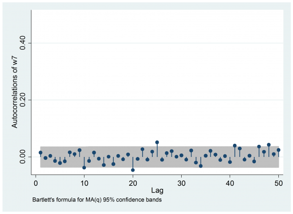
Most importantly, the autocorrelation is negligible, so we have the equivalent of a random sample.
I hit one other problem. Stan wrote all of the parameters to the output file and there are so many that neither Excel nor Stata could cope. So to obtain the estimate of w7 I had to open part of the output file in Excel and then manually copy and paste the relevant columns into Stata.
This particular model creates estimates for every treatment comparison in every study. Hence the huge output file. I suspect that it would be possible to reparameterize the model with far fewer active parameters, which might greatly improve the performance of Stan. One of the difficulties that Stan had in this example is that the code that I wrote is based on a structure and parameterization that was intended for OpenBUGS.
For me, there is no clear winner even though Stan was much slower. I have been using WinBUGS for years and I know more or less how to write efficient WinBUGS code. Perhaps I need to put the same investment into Stan before I will be in a position to judge how good it is.
If you want to download any of the programs referred to in this posting they are available from my webpage at https://www2.le.ac.uk/Members/trj


 Subscribe to John's posts
Recent Comments