Solutions to the Exercises: Chapter 3 – Question 2

Last time I presented my solution to the first question at the end of chapter 3 of ‘Bayesian analysis with Stata’ and this time I want to consider question 2 from the same chapter.

Question 2

This question analyses some data on the prevalence of very pre-term births (VPT) in Europe using a small 1997 survey as the basis for creating the prior in the analysis of a larger study conducted in 2003. The calculations are simple but illustrate how Bayesian analyses can provided information that is simply unavailable using traditional methods.

(i) Use a binomial model for the total number of VPT births in 2003. Base your prior for the binomial parameter, p, on the 1997 survey and approximate it by a suitable beta distribution. Use a Metropolis-Hastings algorithm to derive the posterior for p.

The earlier survey covered two regions and so produced two estimates of the proportion of VPT births; Nord-du-Calais 820/54815 = 0.015 and Trent 1149/59394 = 0.019.

There are two priors that we might want to specify,
(a) the VPT probability in a randomly chosen region of Europe in 2003
(b) the VPT probability for the whole of Europe in 2003
A third possibility is to produce a prior for a specific region in 2003 but this would require more detailed knowledge of that region than I have and so I will not attempt that.

We are asked for prior (b) but it is instructive to consider them both. Of course, these priors are subjective and here you are getting my opinion.

I based my prior on the two earlier surveys together with the article
Tucker & McGuire
Epidemiology of preterm birth
BMJ. 2004; 329(7467): 675–678

The BMJ article tells me that the proportion of pre-term births had increased slightly over the previous 20 years but that the VPT birth rate stayed fairly constant at between 1-2%. The rates being slightly higher in the USA (1.9%) than in Europe. Factors influencing the preterm rates include the frequency of multiple births, the impact of assisted reproduction, the trend towards more obstetric intervention and better measurement of the gestational age through ultrasound rather than menstrual period date.
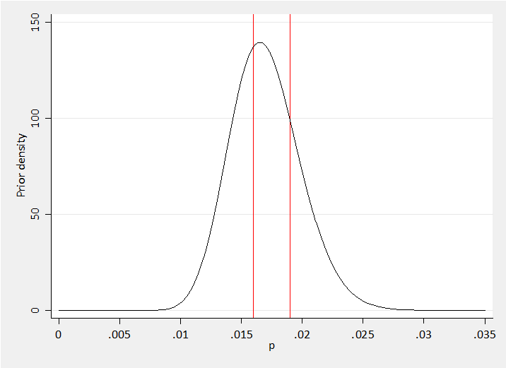
For a randomly chosen region of Europe, I decided that I believed that the proportion of VPT births will turn out to be between 0.010 and 0.025, perhaps Beta(34,1966) which has a mean of 0.0170 and a standard deviation of 0.0029.

My prior for a random region is shown below with the earlier proportions for Nord-du-Calais and Trent shown in red,

twoway function y= betaden(34,1966,x), range(0 0.035)  xlabel(0(0.005) 0.035) ///
xtitle(p) ytitle(Prior density) xline(0.016 0.019,lcol(red))

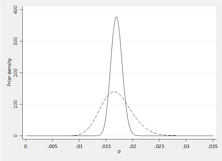
The sample that we want to analyse covers much more of Europe and consists of the combined results for 10 regions, so for consistency we ought to have a mean around 0.0170 and a standard deviation of about 0.0029/sqrt(10)=0.0009. I decided on Beta(255,14745) which has a mean of 0.0170 and st dev of 0.0011.

Here is my prior for all Europe together with my earlier prior for a single region shown as a dashed line.
twoway (function y= betaden(255,14745,x), range(0 0.035) ) ///
(function y= betaden(34,1966,x), range(0 0.035) lpat(dash) ) , ///
xlabel(0(0.005)0.035) xtitle(p) ytitle(Prior density) leg(off)

The second survey gives us the observation of 6533 VPT births out of 497482 live births. First we need a program to calculate the log-posterior.

program logpost
args logp b

local p = `b'[1,1]
scalar `logp’ = 6533*log(`p’)+490949*log(1-`p’) ///
+ 254*log(`p’) + 14744*log(1-`p’)
end

In this program I have chosen not to use logdensity but rather to program the calculations directly. You could of course use
scalar `logp’ = 0
logdensity binomial `logp’ 6533 490949 `p’
logdensity beta `logp’ `p’ 255 14745

A by-product of writing the log-posterior as a direct calculation is that it makes it obvious that the problem is conjugate and by simple addition we can see that the log-posterior is,
6787log(p)+505693log(1-p)
and so the posterior must be Beta(6788,505694) and the posterior mean is 6788/(6788+505694)=0.01325 and the posterior st dev is 0.0001597.

Despite knowing the exact form of the posterior, we are asked to obtain it using a Metropolis-Hastings algorithm.

set seed 950274
matrix b = 0.017
mcmcrun logpost b using temp.csv, replace ///
sampler( mhslogn , sd(0.1) ) burnin(1000) update(5000) par(p) jpost
insheet using temp.csv, clear
gen pc = 100*p
mcmcstats pc

----------------------------------------------------------------------------
 Parameter n    mean     sd    sem median    95% CrI
 ----------------------------------------------------------------------------
 pc        5000 1.325 0.017 0.0007 1.324 ( 1.294, 1.354 )
 ----------------------------------------------------------------------------

I have given the results on a percentage scale so that we can see more of the significant figures. The accuracy of the MCMC algorithm is near perfect for the mean and only slightly high for the st dev.

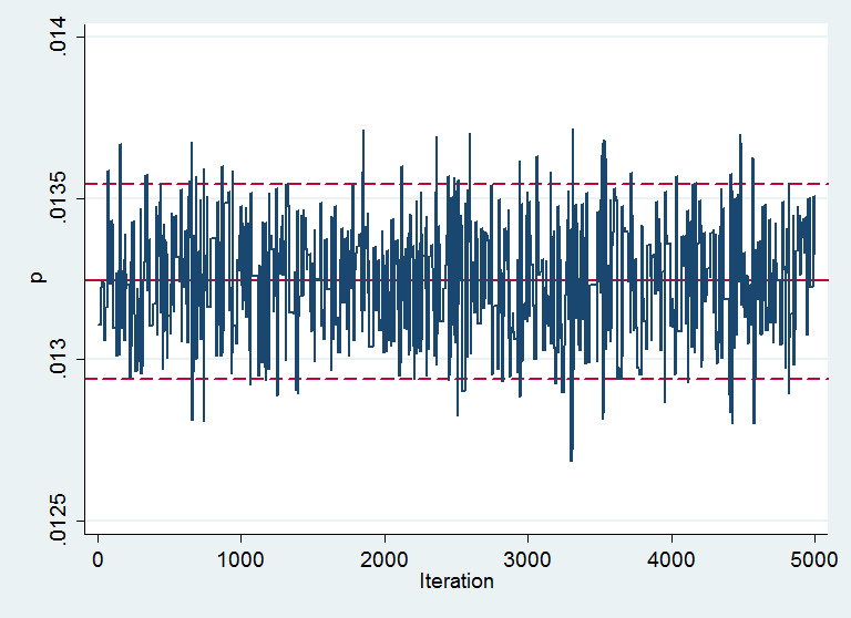
Mixing looks reasonable and there does not appear to be any drift. In fact the plot is a little deceptive because out of 5000 simulations, 4197 were identical with the one before, showing that the chain rejects too many values. This suggests a smaller proposal standard deviation.

Changing the proposal standard deviation to 0.025 reduces the standard error and the standard deviation is more accurate but in truth the improvement is unlikely to be of practical importance, which illustrates the robustness of the Metropolis-Hastings sampler to the choice of the proposal distribution.

----------------------------------------------------------------------------
Parameter n    mean     sd    sem median    95% CrI
 ----------------------------------------------------------------------------
 pc       5000 1.325 0.016 0.0005 1.325 ( 1.294, 1.355 )
 ----------------------------------------------------------------------------

On a log-scale the posterior 95%CrI has a range of log(0.01355)-log(0.01294)=0.046, so we have confirmed that a good proposal standard deviation is about half of this range.

You have probably noticed that my B(255,14745) prior was not such a good a guess. I thought that the level would be about 1.7% and it turned out to be closer to 1.3%. Fortunately the actual data come from a survey of 497,482 live births while my prior was the equivalent of the imagined results from a survey of 15,000 live births, so the prior was not very influential.

(ii) Prepare a program that estimates within the same iteration of the Metropolis-Hastings algorithm all 10 region-specific estimates of p. Run an MCMC analysis using this program

For this question we do need a separate prior for each region but as I have no particular knowledge about the regions I will use my B(34,1966) prior for all of them.

clear
set obs 10
input n y
60444 743
34065 381
84867 1202
52078 724
51939 569
48235 513
43188 566
35336 369
56990 949
30329 517

program logpost
args logp b i

local p = `b'[1,`i’]
scalar `logp’ = y[`i’]*log(`p’)+(n[`i’]-y[`i’])*log(1-`p’) ///
+ 33*log(`p’) + 1965*log(1-`p’)
end

set seed 950274
matrix b = J(1,10,0.017)
mcmcrun logpost b using temp.csv, replace ///
sampler( 10(mhslogn , sd(0.025)) ) burnin(1000) update(5000) ///
par(p1-p10)
insheet using temp.csv, clear
forvalues i=1/10 {
gen pc`i’ = 100*p`i’
}
mcmcstats pc*

----------------------------------------------------------------------------
 Parameter n  mean    sd    sem median    95% CrI
 ----------------------------------------------------------------------------
 pc1    5000 1.243 0.044 0.0022 1.243 ( 1.159, 1.326 )
 pc2    5000 1.153 0.056 0.0037 1.152 ( 1.054, 1.268 )
 pc3    5000 1.424 0.040 0.0017 1.423 ( 1.349, 1.506 )
 pc4    5000 1.408 0.053 0.0028 1.406 ( 1.312, 1.514 )
 pc5    5000 1.120 0.044 0.0023 1.119 ( 1.037, 1.208 )
 pc6    5000 1.093 0.046 0.0027 1.093 ( 1.006, 1.185 )
 pc7    5000 1.331 0.054 0.0030 1.330 ( 1.224, 1.444 )
 pc8    5000 1.082 0.053 0.0035 1.080 ( 0.982, 1.194 )
 pc9    5000 1.666 0.052 0.0024 1.665 ( 1.568, 1.767 )
 pc10   5000 1.708 0.070 0.0038 1.709 ( 1.572, 1.841 )
 ----------------------------------------------------------------------------

(iii) Estimate the probability that the Trent region of the UK has the highest rate of VPT births out of the 10 regions

Trent is region 10 in the list above and does indeed have the largest posterior mean but the uncertainty is such that it is possible that region 9 or even one of the others has a higher probability of VPT births.
egen mp = rmax(pc1-pc9)
count if pc10 > mp
and we find that 3422 out of the 5000 simulations placed Trent with the highest VPT percentage. So the estimated probability that Trent has the highest probability is 0.68.

Questions like this are of real interest but they simply cannot be answered by non-Bayesian methods that concentrate on P(Data|Model) rather than P(Model|Data).

(iv) Estimate the probability that the parameter p for Flanders is higher than that for Trent

Flanders is region 1 and pc1 was never larger than pc10 so the estimated probability that Flanders has a higher rate than Trent is zero.

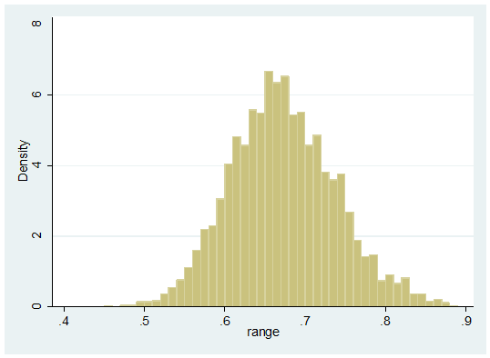
(v) Estimate the range of values of p across the 10 regions. Plot a histogram of the ranges. Does this distribution demonstrate that the values of p are not the same in every region?

. egen rmx = rowmax(pc1-pc10)
. egen rmn = rowmin(pc1-pc10)
. gen range = rmx – rmn

Gives an average range of about 0.65%. However, to choose properly between the two models (varying p and common p) we should use the methods of Chapter 10 where we address the question of model choice. Here we have only seen results under one of those models so we should not jump to conclusions. Model choice requires us to compute P(Data|Model) for different models, what we have calculated is just the marginal posterior distribution of the range of the pc’s.

With hindsight this question is too simple and would benefit from the addition of a more difficult final part, perhaps replacing (iv). Maybe the reader could be required to fit a hierarchical model in which the distribution of the region-specific probabilities of VPT birth follows a Beta distribution, B(a,b), and the prior is placed on a and b. Such a model is slightly more challenging to fit although the hardest part of the question would be to set an appropriate prior on (a,b) since it would not make sense to treat a and b as independent.