This is another of my occasional postings working through the exercises given at the end of the chapters in ‘Bayesian analysis with Stata’.
Chapter 3 introduces the Metropolis-Hastings sampler and so enables us to tackle any small sized Bayesian analysis. For larger problems this method can be too slow and faster algorithms are needed. Despite this, an analysis with a Metropolis-Hastings sampler can be used to illustrate most of the important issues that arise with the MCMC method. Because there is so much to say, I will only answer question 1 in this posting and I’ll consider question 2 next time, which will be in two weeks as I am about to take some leave.
Question 1 extends the example considered in the text that looked at polyp counts in women taking part in a colon cancer prevention trial. In the question we are asked to repeat the analysis for men.
We are told to use a gamma(3,0.3) prior for the average rate, λ, and to fit the zero-truncated Poisson distribution to the trial data on the men using a Metropolis-Hastings algorithm with a log-normal random walk proposal distribution.
(i) Asks us to identify a good value for the proposal standard deviation and a suitable length of burn-in
My data file contains the data for men and women, so I just keep the data on men and have,
gender y f
 Male 1 434
 Male 2 178
 Male 3 87
 Male 4 40
 Male 5 23
 Male 6 12
 Male 7 7
 Male 8 4
 Male 9 1
 Male 10 3
I’ve set a seed so that anyone can reproduce my answers exactly, but this is not normal practice and we must accept that with any simulation based method there will be an element of random variation in the answer. If I were to use this question as a student exercise, I would want the students to start with different seeds so that we could compare their answers. This would help them to understand the importance of running the chain for long enough.
The model is the same one that was used for the women in the text of chapter 3 so the program logpost is identical, except that the total number of men is 789. Logpost calculates the log-likelihood and combines it with a gamma prior on the parameter lambda. My call to mcmcrun does not request a burnin so we store the chain from its initial value of lambda=1. The log-scale Metropolis-Hastings sampler is used because lambda must be positive and I have chosen a sd of 0.05 for the proposal distribution based on our experience of analysing the women.
use “polyp.dta”, clear
keep if gender == “Male”
set seed 456901
program logpost
args logp b
local lambda = `b'[1,1]
scalar `logp’ = 0
logdensity poisson `logp’ y `lambda’ [fw=f]
scalar `logp’ = `logp’ – 789*log(1-exp(-`lambda’))
logdensity gamma `logp’ `lambda’ 3 0.3
end
matrix b = ( 1 )
mcmcrun logpost b using temp.csv, samp(mhslogn , sd(0.05)) ///
burn(0) update(1000) replace par(lambda) jpost
insheet using temp.csv, clear
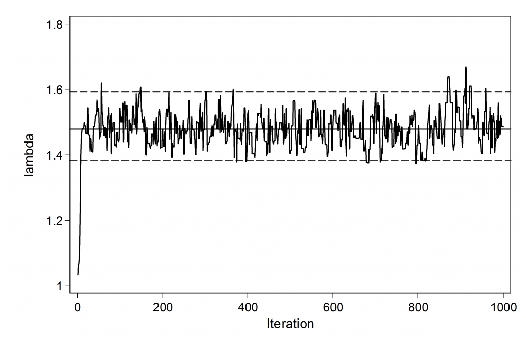
mcmctrace lambda, gopt(scheme(lean1))
This short run suggests that a burn-in of 200 would be ample for use with a starting value of 1.0. Mixing is not bad so the choice of proposal standard deviation looks reasonable. We can count the number of rejected moves between updates 201 and 1000 using
. count if lambda == lambda[_n-1] & _n > 200
This gave me the value 327, so around 327/800 or 41% of the proposals are rejected. The guideline is to reject a little over half of the proposals so perhaps we could increase the proposal standard deviation a little but this is not going to make much difference. Another resaonable approach would be to set the adapt option with mcmcrun in order to learn about the proposal standard deviation during the burn-in.
(ii) Asks us to run the algorithm five times with a run length of 5,000 after the burn-in and note the posterior mean estimate of λ. Are the results consistent to two decimal places? Find the smallest run length that will give two decimal places of accuracy.
Here is some code that performs the analysis. Once again I have set a seed so that you can reproduce my results.
set seed 456901
forvalues i=1/5 {
quietly {
use “polyp.dta”, clear
keep if gender == “Male”
matrix b = ( 1 )
mcmcrun logpost b using temp.csv, samp(mhslogn , sd(0.05)) ///
burn(200) update(5000) replace par(lambda) jpost
insheet using temp.csv, clear
mcmcstats lambda
}
di %8.4f r(mn1) %8.4f r(sd1) %8.4f r(se1)
}
The displayed results are,
Mean St Dev SEM
1.4852 0.0510 0.0017
1.4904 0.0517 0.0017
1.4871 0.0501 0.0016
1.4871 0.0519 0.0018
1.4858 0.0481 0.0015
So each of the posterior mean estimates of lambda rounds to 1.49 and so they are consistent to 2 decimal places. Notice that the posterior standard deviation varies between 0.048 and 0.052 so it is stable to two decimal places but not to two significant figures. It is generally the case that you need more simulations to obtain consistent standard deviations.
Had the chain been independent the standard error would have been around 0.051/sqrt(5000) = 0.0007 so the correlation in the chain has roughly doubled the standard error. An observed standard error of 0.0017 means an accuracy of ±0.0034, which confirms that the results ought to be consistent to within 2 decimal places. As a rough guide we might assume that for results to be accurate to 2 dec places we need the accuracy to be ±0.005 or the sem to be smaller than 0.0025. This suggests that we could have got away with a smaller number of iterations of the sampler. 5000*0.00172/0.00252 = 2300. So perhaps 2,500 would have been enough.
Re-running the analysis with 2500 updates we get,
1.4852 0.0520 0.0024
1.4861 0.0506 0.0024
1.4909 0.0509 0.0023
1.4872 0.0492 0.0022
1.4843 0.0490 0.0021
This (almost) confirms our approximate calculations. The answer seems to be about 1.487 so we need to do slightly better than ±0.005 in order to get 2 dec places of accuracy.
(iii) Asks us to check the sensitivity of the estimate of λ to the choice of the prior by contrasting gamma(3,0.3), gamma(6,0.15) and gamma(1.5,0.6)
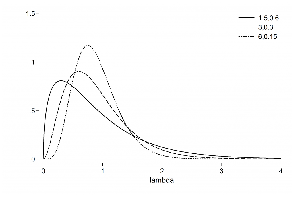
Let’s start by picturing the three priors.
twoway ( function y=gammaden(1.5,0.6,0,x), range(0 4) ) ///
( function y=gammaden(3,0.3,0,x), range(0 4) ) ///
( function y=gammaden(6,0.15,0,x), range(0 4) ) , scheme(lean1) ///
xtitle(lambda) ytitle(” “) ///
leg( ring(0) pos(1) label(1 “1.5,0.6”) label(2 “3,0.3”) label(3 “6,0.15”))
The means of the priors are all 0.9 but the variances and the modes change.
Now let’s re-run the analyses with the different priors. The code is as for part (i) except that I chose a burn-in of 200 a run length of 5,000 and, of course, I changed the priors. Each time I set the seed to 456901 to make my results reproducible.
G(1.5,0.6)
 --------------------------------------------------------
 Parameter n mean   sd    sem    median    95% CrI
 --------------------------------------------------------
 lambda 5000 1.486 0.051 0.0016 1.487 ( 1.389, 1.592 )
 --------------------------------------------------------
G(3,0.3)
 --------------------------------------------------------
 Parameter n mean   sd    sem    median    95% CrI
 --------------------------------------------------------
 lambda 5000 1.485 0.051 0.0017 1.485 ( 1.386, 1.591 )
 --------------------------------------------------------
G(6,0.15)
 --------------------------------------------------------
 Parameter n mean   sd    sem    median    95% CrI
 --------------------------------------------------------
 lambda 5000 1.490 0.051 0.0017 1.491 ( 1.392, 1.596 )
 --------------------------------------------------------
The priors show no effect on the second decimal place, i.e. no practical importance
Had we needed 3 dec places of accuracy we would have required a sem=0.00025 so the run length would need to be 5000*0.00172/0.000252 = 230,000
I re-ran the analysis with 250,000 iterations and obtained,
 G(1.5,0.6)
  --------------------------------------------------------
 Parameter n mean sd sem median 95% CrI
  --------------------------------------------------------
 lambda 250000 1.489 0.051 0.0002 1.488 ( 1.390, 1.589 )
  --------------------------------------------------------
 G(3,0.3)
  --------------------------------------------------------
 Parameter n mean sd sem median 95% CrI
  --------------------------------------------------------
 lambda 250000 1.487 0.051 0.0002 1.487 ( 1.389, 1.587 )
  --------------------------------------------------------
 G(6,0.15)
  --------------------------------------------------------
 Parameter n mean sd sem median 95% CrI
  --------------------------------------------------------
 lambda 250000 1.492 0.051 0.0002 1.492 ( 1.394, 1.592 )
  --------------------------------------------------------
So the priors do affect the third decimal place in the posterior mean. It is very unlikely that such a difference would ever be of practical importance.
I hope that this example serves to demonstrate that we should not be too fussy about the priors that we use. Unless the sample size is small, we can change the prior slightly without having any meaningful impact on the answer. Remember too that ‘all models are wrong’ and small changes to the model are likely to have at least as strong an impact as any approximation in the prior.
(iv) Asks us to analyse the data on men and on women under a zero-truncated Poisson model in order to decide whether the average rate of polyps varies by gender.
As the two models are unrelated to one another we could analyse them separately but, for no special reason, I have decided to calculate a single joint posterior. The answer will be the same.
program logpost
args logp b
local lambdaM = `b'[1,1]
local lambdaF = `b'[1,2]
scalar `logp’ = 0
logdensity poisson `logp’ y `lambdaM’ [fw=fM]
scalar `logp’ = `logp’ – 789*log(1-exp(-`lambdaM’))
logdensity gamma `logp’ `lambdaM’ 3 0.3
logdensity poisson `logp’ y `lambdaF’ [fw=fF]
scalar `logp’ = `logp’ – 390*log(1-exp(-`lambdaF’))
logdensity gamma `logp’ `lambdaF’ 3 0.3
end
matrix b = ( 1 , 1 )
mcmcrun logpost b using temp.csv, samp( 2(mhslogn , sd(0.05)) ) ///
burn(200) update(5000) replace par(lambdaM lambdaF) jpost
insheet using temp.csv, clear case
mcmcstats lambdaM lambdaF
kdensity lambdaM , gen(xM yM) nograph
kdensity lambdaF , gen(xF yF) nograph
twoway (line yM xM) (line yF xF) , leg(ring(0) pos(11) col(1) ///
label(1 “Male”) label(2 “Female”))
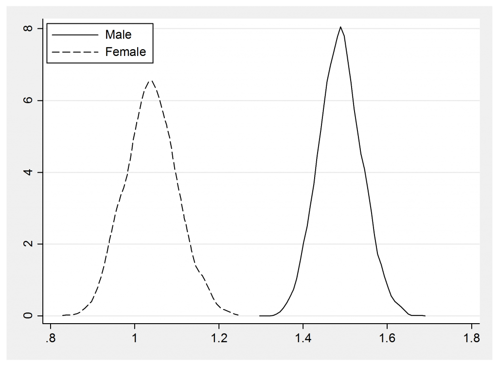
The summary statistics show the large difference between men and women
 --------------------------------------------------------
 Parameter n    mean sd     sem   median    95% CrI
 --------------------------------------------------------
 lambdaM 5000 1.489 0.052 0.0017 1.489 ( 1.390, 1.594 )
 lambdaF 5000 1.039 0.062 0.0028 1.039 ( 0.922, 1.167 )
 --------------------------------------------------------
and this impression is reinforced by the posterior density plots

I
Another way to illustrate the difference would be to calculate the difference between the two lambdas and summarize its posterior, which is positioned well away from zero. The probability that delta<0 would be a good summary statistic for this analysis, except that the effect is so clear cut that the probability is indistinguishable from zero.
gen delta = lambdaM – lambdaF
mcmcstats delta
------------------------------------------------------
 Parameter n mean    sd   sem   median     95% CrI
 -----------------------------------------------------
 delta 5000 0.449 0.079 0.0030 0.448 ( 0.295, 0.602 )
 -----------------------------------------------------
(v) The zero-truncated Generalized Poisson model is able to allow for clustering of polyps within susceptible individuals. Investigate this model by running a joint analysis of the data on men and women in which men and women have different means μm and μf but the same amount of clustering α. Set your own realistically vague priors. Investigate the posterior of μm-μf.
For some reason I called these parameters mu in the question where before I referred to lambda. Perhaps I will change the wording if the book is ever re-printed. Anyway I will stick with lambda in my answer.
My priors on both λ’s are gamma G(3,0.3) and for alpha G(0.5,2). I have used a block updating algorithm. The burn-in is 1,000. The run length is 20,000 but the run is thinned by 4 to give 5,000 values.
program logpost
args logp b
local lambdaM = exp(`b'[1,1])
local lambdaF = exp(`b'[1,2])
local alpha = exp(`b'[1,3])
local thetaM = `lambdaM’/(1+`alpha’*`lambdaM’)
local thetaF = `lambdaF’/(1+`alpha’*`lambdaF’)
tempvar ay lnp
gen `ay’ = 1+ `alpha’*y
gen `lnp’ = y*log(`thetaM’)+(y-1)*log(`ay’)-`thetaM’*`ay’-log(1-exp(-`thetaM’))
qui su `lnp’ [fw=fM]
scalar `logp’ = r(sum)
replace `lnp’ = y*log(`thetaF’)+(y-1)*log(`ay’)-`thetaF’*`ay’-log(1-exp(-`thetaF’))
qui su `lnp’ [fw=fF]
scalar `logp’ = `logp’ + r(sum)
logdensity gamma `logp’ `lambdaM’ 3 0.3
logdensity gamma `logp’ `lambdaF’ 3 0.3
logdensity gamma `logp’ `alpha’ 0.5 2
scalar `logp’ = `logp’ + `b'[1,1] + `b'[1,2] + `b'[1,3]
end
matrix b = (1.0 , 1.0, 0.1)
matrix V = (.11, 0.055, -0.120\ 0.055, 0.110, -0.120 \ -0.120, -0.120, 0.200)
matrix L = cholesky(V)
mcmcrun logpost b using temp.csv, samp( mhsmnorm ,c(L) ) ///
burn(1000) update(20000) thin(4) replace par(logM logF logalpha) jpost
insheet using temp.csv, clear case
mcmcstats logM logF logalpha , corr
graph matrix logM logF logalpha
gen lambdaM = exp(logM)
gen lambdaF = exp(logF)
gen alpha = exp(logalpha)
gen delta = lambdaM – lambdaF
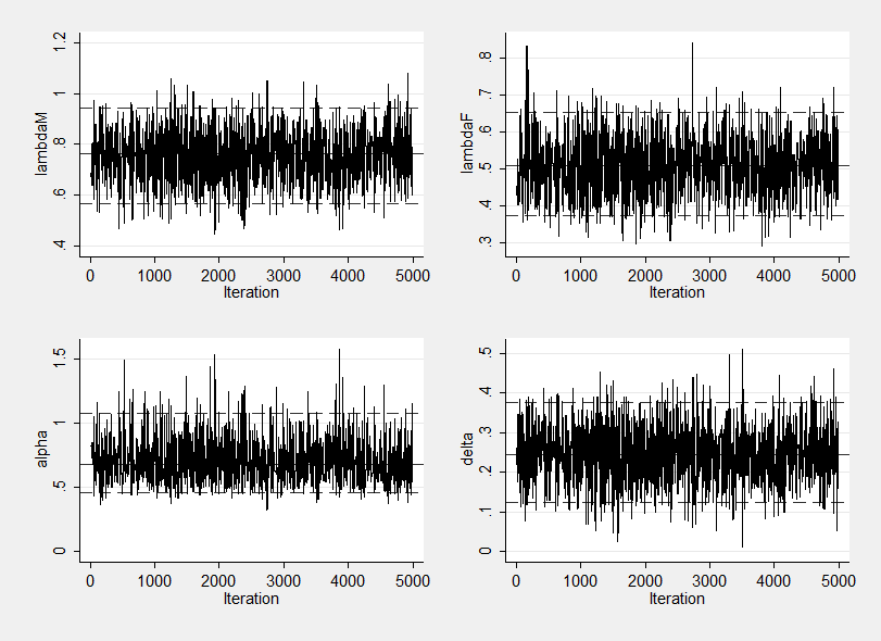
mcmctrace lambdaM lambdaF alpha delta
mcmcstats lambdaM lambdaF alpha delta, corr
You might well come up with a different algorithm that works perfectly well, so I think that I should justify my choice.
Looking at figure 3.5 in Chapter 3, which shows lambda against alpha for the women alone, we can see that these two parameters are quite strongly negatively correlated. This suggests that updating one parameter at a time will be inefficient.
The Metropolis-Hastings block updater introduced in chapter 3 is based on a multivariate normal distribution, which is not ideal for this problem because we want all three parameters to be positive by definition. The multivariate normal proposals could have problems if the chain got close to zero. In fact with this problem all three parameters are clearly non-zero so we could probably get away without any transformation, but I decided to work in terms of the logs of the parameters to protect myself from the remote possibility of getting close to zero.
For the multivariate normal proposals to work well I have to make a guess at the covariance matrix of the logged parameters. From the analysis of the women shown in on figure 3.5 from chapter 3 I expected the posterior distribution of lambdaF to range from about 0.3 to 0.9, on a log-scale this is -1.30 to -0.11, a range of 1.19. So the standard deviation must be about a quarter of this range or 0.30 and the variance about 0.09. In a similar way I guessed that alpha would be between 0.2 and 1.2 so I guessed a variance of 0.20 for log(alpha). I then assumed a negative correlation of -0.8 between log(alpha) and both log(lambda) and a positive correlation of +0.5 between log(lambdaF) and log(lambdaM) induced by their common dependence on alpha. These guesses can be very rough and the sampler will still work efficiently.
This covariance matrix is called V in the code.
Inside the program logpost, I undo the log-scales by taking exponents and then calculate the log-posterior in the usual way. The final line of the code adds the Jacobian to allow for the change of scale.
The log(parameters) have summary statistics
----------------------------------------------------------------------------
Parameter         n     mean       sd      sem   median         95% CrI
----------------------------------------------------------------------------
 logM          5000   -0.289    0.131   0.0040   -0.272 (  -0.565,  -0.060 )
 logF          5000   -0.686    0.147   0.0045   -0.676 (  -0.989,  -0.426 )
 logalpha      5000   -0.377    0.219   0.0070   -0.389 (  -0.783,   0.069 )
----------------------------------------------------------------------------
Correlations
(obs=5000)
             |     logM     logF logalpha
-------------+---------------------------
        logM |   1.0000
        logF |   0.7511   1.0000
    logalpha |  -0.9042  -0.8207   1.0000
So my guesses at the correlations were quite good. Transforming onto a more interpretable scale the summaries are
 ----------------------------------------------------------------------------
Parameter         n     mean       sd      sem   median         95% CrI
----------------------------------------------------------------------------
 lambdaM       5000    0.755    0.097   0.0029    0.762 (   0.568,   0.941 )
 lambdaF       5000    0.509    0.074   0.0023    0.509 (   0.372,   0.653 )
 alpha         5000    0.703    0.159   0.0050    0.678 (   0.457,   1.072 )
 delta         5000    0.246    0.065   0.0019    0.244 (   0.125,   0.376 )
----------------------------------------------------------------------------
There does seem to be good evidence of clustering and allowing for that clustering, the Poisson means for both men and women are roughly halved although there is still good evidence that men and women differ.
Mixing seems quite good. The standard errors are quite small (random sampling would have given 0.1/sqrt(20000)=0.0007 and even with thinning we have a se of 0.0029) and the trace plots show no drift and seem to cover the posterior well.
And the matrix scatter plots of the chains illustrate why an algorithm that updated one parameter at a time would have taken longer to converge.
Here I used my guess at the covariance matrix of the posterior distribution, V, as the covariance matrix of the multivariate normal proposals. You can make the algorithm slightly more efficient by scaling this matrix slightly, perhaps basing the proposals on V/4 rather than V. You could even optimise the scaling factor by learning about it during the burn-in.


 Subscribe to John's posts
Recent Comments