Back to Google Flu Trends

It has been rather a long gap since my last posting but I am told that the re-direction virus has been cleared from the host’s server so I am going to return to the topic of fitting Bayesian models to flu epidemics using the Google Flu Trends data (https://en.wikipedia.org/wiki/Google_Flu_Trends). Google’s project created estimates of the number of cases of influenza-like illness each week  based on the number of internet searches of flu related terms. You can read my previous postings on this topic here and here.

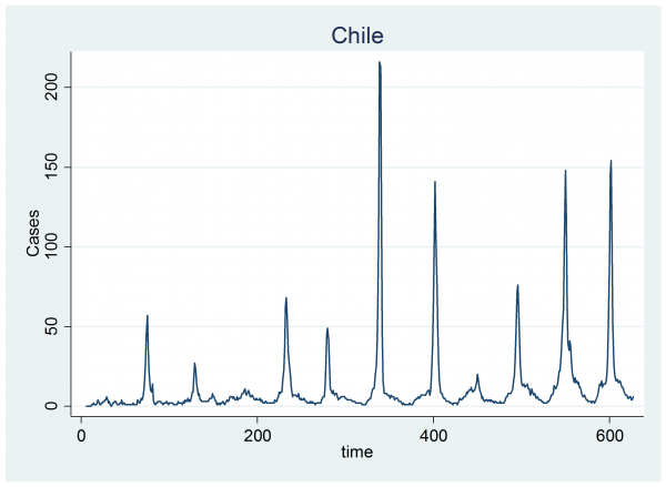
To recap, we were analysing the weekly data from Chile

In the graph you can see that the number of cases rises slightly during the winter and falls back to zero in the summer. On top of that cyclical pattern there are winter spikes of varying intensity and duration that represent the flu epidemics. The model for these data assumes that the number of cases follows a Poisson distribution and that each year the log of the expected number of cases, mu, is made up of a sine wave plus a random jump, H_i, in the level that has a starting week, S_i, and a finishing week, E_i.

log(mu) = a + b time/1000 + c sin(0.060415*week) + H_iδ(year==i & week>=S_i & week<=E_i)

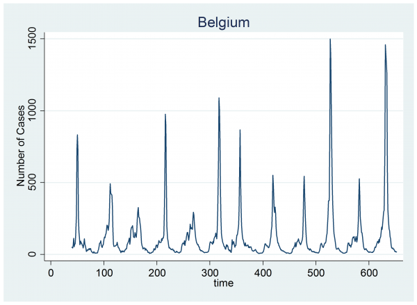
The model was quite successful at capturing the epidemics in Chile so now we will look at the data for another country. I’ve chosen Belgium because its epidemics are fairly clear, just as they are in Chile, but also because year 3 in Belgium shows the suggestion of a second peak that occurs prior to the main flu epidemic.

We can fit the same Bayesian model to these data using the code that I gave before, provided that we adjust the definitions of weeks and years to reflect the fact that Belgium is in the Northern Hemisphere and its summer minimum occurs in the middle of a conventional year. To make life easier for myself, I have defined my years to start on the 1st of July.

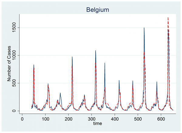
With this modification we can fit the model exactly as before. The plot below shows the same data together with a red line representing the model fit created from the posterior means for each parameter. On the whole the Bayesian algorithm has again performed well.

However, look carefully at year 3. The algorithm has picked up the minor peak and failed to find the larger one. This suggests that we have two problems.

Firstly, we need to improve the mixing so that the chain can move between peaks within the same year. This would mean trying bigger jumps in the location of the epidemic with the start and end times both moving together. To achieve this it might be easier to parameterize in terms of the start and the length of the epidemic rather than the start and the end.

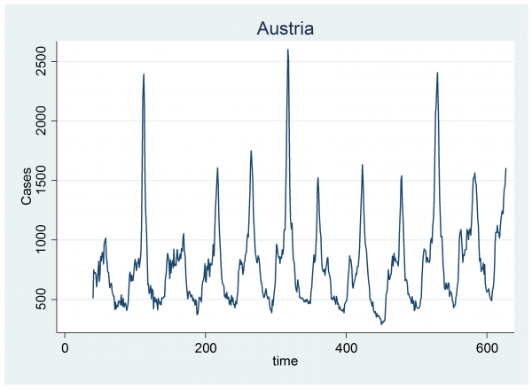
The second problem is even more fundamental. Some years appear to have two genuine epidemics and our model only allows for one. Look at the data for Austria. It appears that there are often two spikes in a year, one small and one large.

One might argue whether or not the second peak reflects a pattern in influenza or a pattern in internet use, but our job is to explain these data and at present we are not able to represent this pattern.

There are various ways of adapting the model to allow for a second peak. We might, for example, fit a model that has 2 epidemics every year and rely on the size of the second spike to be small in years with only one epidemic.

Such a model would be a little untidy because the position of the non-existent epidemics would be very poorly defined and mixing would be a problem. What is more, when we came to analyse the results we would have to pick an arbitrary spike height and declare spikes smaller than that to be non-existent or false epidemics. The choice of this cut-off value would be very difficult to justify. It just does not feel Bayesian.

A better solution would be to allow the number of epidemics each year to be a parameter in the model that we could estimate as part of the chain. Then the analysis would control whether or not a small spike stays in the model. Small spikes might come and go in the chain and the proportional of the time that two spikes are present would give us an estimate of the probability that there were two real epidemics that year.

This approach would be neater but it creates a problem. The MCMC chain will need to jump between solutions that have different numbers of epidemics and, as each epidemic has a height, a start and an end, it follows that whole sets of parameters will drop out of the model when we jump to a solution with a smaller number of spikes and those sets of parameters will re-appear when we jump to a solution with extra spikes.

Rather than think of this situation as a single model in which the number of parameters changes, it is simpler to think of it as a large set of  models each with a fixed number of parameters. Our job is both to select the best model and to estimate its parameters, although as Bayesians we will acknowledge uncertainty over which model is actually the best.

We have 12 years of data from Belgium and each year can have 0, 1 or 2 epidemics, so we are left to choose between 3¹²=531,441 different models. Each epidemic has a start, an end and a height, so the model without any epidemics will have 0 spike parameters and at the other extreme the model with 2 epidemics every year will have 12*3*2=72 spike parameters. Somehow, we must jump randomly between the 531,441 models, changing the parameters as we move.

The most commonly used Bayesian algorithm for moving between models with different parameterizations is called Reversible Jump Markov chain Monte Carlo (RJMCMC). This algorithm is very important in statistics because it is needed for a wide range of problems in which the exact form of the model is not known in advance.

Think of all of the regression models that you have fitted in which you did not know at the outset which covariates needed to be included.

When I was writing the book, Bayesian Analysis with Stata, I considered putting in a chapter on RJMCMC but in the end decided that it would take too much space to cover the topic properly, so it got left out. Now we need it.