
Last time, I showed how we can write R code for fitting a Bayesian Generalized Linear Mixed Model and insert it into a Stata do file, so that the computation is performed by the R program, MCMCglmm, while the results are available in Stata. The drawback of that approach is that it requires the user to understand the R syntax. This week, I am going to present a Stata command that writes the R code automatically so that a Stata user can fit models without knowing anything about R.
Rather than work through the code in the ado file that defines the command, I want to concentrate on some examples of its use, so I will give only the briefest description of how it works.
The R code for using MCMCglmm follows the same pattern for every model except for specific options such as, the distribution, the explanatory variables, the length of the MCMC chain and the structure of the random effects. So I have produced a template called rtmcmcglmm.txt that I store in a subdirectory of my PERSONAL folder called RTEMPLATES. This template includes the R code for calling MCMCglmm, except that where there is something that might change, I replace it with an @. Then I have an ado file called rtemplates.ado that re-writes the file inserting specified items where it finds an @.
My command mcmcglmm.ado can be called from Stata and works out the required items for inserting into the template based on Stata options set by the user. So, to the user, it looks like any other Stata command.
I have taken my examples from Sophia Rabe-Hesketh and Anders Skrondal’s book entitled, Multilevel and Longitudinal Modelling using Stata. I only have the one volume, original edition but I believe that MCMCglmm will fit every model covered in that book and a great many more besides. It also has the added advantage of providing Bayesian fitting so we have the choice of either setting informative priors, or of getting very close to the ML solution by setting vague priors. However, nothing is perfect and in these examples we will see some of the problems with MCMCglmm.
Let’s start with a very simple linear model with normal errors and a random intercept. The book illustrates this situation with some data on qualifications obtained by 4059 children from 65 schools in inner-London. The data are available to download from http://www.stata-press.com/data/mlmus/gcse
In the data there is a standardised qualification score, gcse, that was measured at age 16 and an explanatory variable, lrt, that is a standardised reading score from when the children started at the school aged 11.
In the random intercept model we imagine that the average gcse score will vary between schools for all sorts of reasons, such as the quality of the teaching and the average socio-economic background of the children. Since these factors are unmeasured, we allow for them through a random intercept with a different value for each school.
To analyse these data with MCMCglmm’ s default of very vague priors we could use the Stata program,
use http://stata-press.com/data/mlmus/gcse, clear
saveold gcse.dta , replace version(12)
mcmcglmm gcse lrt, dta(gcse.dta) ///
family(gaussian) burnin(1000) updates(20000) thin(2) ///
random(school) log(log.txt) out(myout.txt)
view log.txt
rextract using myout.txt, item(Sol) clear
rextract using myout.txt, item(VCV) add
rename Sol_1 cons
rename Sol_2 lrt
gen sd_s = sqrt(VCV_1)
gen sd_r = sqrt(VCV_2)
gen rho = VCV_1/(VCV_1+VCV_2)
mcmctrace cons lrt sd_s sd_r
mcmcstats cons lrt sd_s sd_r rho
I was not sure what version of Stata the data were stored under so I read the data and saved it in an old format that R can read. Next I use my mcmcglmm command, which gives the specification of the options a Stata-like feel. The basic model is gcse=cons+lrt, hence these variables follow the command as they would with regress. The dta option allows me to specify the source of the data, we are using normal errors regression so the family is gaussian and I specify the length of the MCMC run. The random term has a different intercept for each school, the summarised results will be sent to log.txt and the raw results will go to myout.txt.
I check the log file with the view command to make sure that there were no problems, then I read the simulated regression coefficients (Sol) and the simulated variances (VCV) from myout.txt as described last week. I do a bit of renaming, I check the traces (mixing is very good so I will not show them) and I summarise the results including the proportion of the variance explained by the random intercept.
-----------------------------------------------------------
 Parameter   n  mean    sd    sem median     95% CrI
 ----------------------------------------------------------
 cons    10000 0.018 0.403 0.0040 0.012 ( -0.767, 0.816 )
 lrt     10000 0.563 0.012 0.0001 0.564 ( 0.539, 0.587 )
 sd_s    10000 3.096 0.320 0.0033 3.075 ( 2.524, 3.776 )
 sd_r    10000 7.525 0.085 0.0009 7.524 ( 7.360, 7.694 )
 rho     10000 0.145 0.026 0.0003 0.143 ( 0.100, 0.202 )
 ----------------------------------------------------------
The results are within sampling error of those given by xtmixed, with the advantage that the credible intervals do not rely on normal approximations. If you want more decimal places of accuracy then just increase the length of the MCMC run.
I have fitted the model as in Multilevel and Longitudinal Modelling using Stata but I think that we would have a strong case for omitting the constant from the model given that y and x are standardised. You could do this with the noconstant option.
mcmcglmm gcse lrt, dta(gcse.dta) nocons ///
family(gaussian) burnin(1000) updates(20000) thin(2) ///
random(school) log(log.txt) out(myout.txt)
The next question to ask is whether the slope really is 0.56 for every school, perhaps performance of children in some schools in more dependent on their ability when they arrive than it is in other schools. Now we want a random intercept and a random slope. I’ll just give the bits of the code that change,
mcmcglmm gcse lrt , dta(gcse.dta) ///
family(gaussian) burnin(1000) updates(20000) thin(2) ///
random(idh(1+lrt):school) log(log.txt) out(myout.txt)
gen sd_s = sqrt(VCV_1)
gen sd_sl = sqrt(VCV_2)
gen sd_r = sqrt(VCV_3)
mcmcstats cons lrt sd_s sd_sl sd_r
To obtain both a random intercept and a random slope we specify
idh(1+lrt):school
which I think is much more intuitive than xtmixed’s
|| school: lrt, cov(ind)
In MCMCglmm’s notation the school random effect acts on intercept (1) and the coefficient (lrt), hence 1+lrt and idh requests independence between the two random effects.
The analysis takes about 30 seconds and gives results equivalent to those provided by xtmixed.
-----------------------------------------------------------
 Parameter   n  mean    sd    sem median     95% CrI
 ----------------------------------------------------------
 cons    10000 -0.077 0.401 0.0040 -0.082 ( -0.862, 0.713 )
 lrt     10000  0.557 0.020 0.0002  0.557 ( 0.517, 0.596 )
 sd_s    10000  3.063 0.317 0.0034  3.040 ( 2.500, 3.743 )
 sd_sl   10000  0.120 0.020 0.0003  0.119 ( 0.085, 0.162 )
 sd_r    10000  7.443 0.085 0.0008  7.443 ( 7.281, 7.611 )
 -----------------------------------------------------------
It is possible, even likely, that the two random effects will not be independent. Schools that do well overall might be more or less influenced by the ability of the children when they start. So it would be interesting to allow the random effects to be correlated. We do this by a simple change to the random option,
us(1+lrt):school
where us stands for unstructured (think USA).
Interestingly the MCMC analysis has trouble differentiating between all of the sources of variance. This is an example where it is better to have realistically vague priors. So I set,
matrix v = (10,0,0.01)
mcmcglmm gcse lrt, dta(gcse.dta) ///
family(gaussian) burnin(1000) updates(20000) thin(2) ///
rprior(V=50 nu=5) gprior(V=v nu=5) ///
random(us(1+lrt):school) log(log.txt) out(myout.txt)
I set the value of nu (my confidence in my guess at the variance) to be quite low so I am still having very little impact on the results, for example my prior says that the residual variance is likely to be between 3 and 845. Even this small guidance is enough to get the algorithm to converge and it gives,
-------------------------------------------------------------
 Parameter   n   mean    sd    sem median   95% CrI
 ------------------------------------------------------------
 cons    10000 -0.108 0.408 0.0041 -0.111 ( -0.921, 0.682 )
 lrt     10000  0.556 0.020 0.0002  0.556 ( 0.516, 0.595 )
 sd_s    10000  3.113 0.308 0.0033  3.093 ( 2.577, 3.772 )
 sd_sl   10000  0.122 0.018 0.0003  0.121 ( 0.090, 0.160 )
 r       10000  0.420 0.142 0.0019  0.432 ( 0.116, 0.667 )
 sd_r    10000  7.442 0.085 0.0008  7.440 ( 7.281, 7.613 )
 -------------- ----------------------------------------------
Once again we are very close to xtmixed’s maximum likelihood solution. You can see the source of the convergence problem by looking at the the choice that I made for the prior variance matrix v that put things right. The variance on the intercept is about 1000 times greater than the variance on the slope. We could have had much the same effect on convergence by scaling lrt differently.
So I tried,
use http://stata-press.com/data/mlmus/gcse, clear
replace lrt = lrt/10
saveold gcse.dta , replace version(12)
mcmcglmm gcse lrt using temp.R, dta(gcse.dta) ///
family(gaussian) burnin(1000) updates(20000) thin(2) ///
random(us(1+lrt):school) ///
log(log.txt) out(myout.txt)
Now there are no convergence issues and (apart from the factor of 10) we get the same answer as xtmixed to within sampling error.
 ----------------------------------------------------------------------------
Parameter    n   mean    sd    sem median    95% CrI
----------------------------------------------------------------------------
 cons    10000 -0.113 0.408 0.0041 -0.113 ( -0.914, 0.681 )
 lrt     10000  5.568 0.206 0.0021  5.569 ( 5.161, 5.971 )
 sd_s    10000  3.092 0.319 0.0034  3.067 ( 2.538, 3.773 )
 sd_sl   10000  1.221 0.203 0.0036  1.213 ( 0.846, 1.643 )
 r       10000  0.506 0.154 0.0024  0.517 ( 0.172, 0.772 )
 sd_r    10000  7.445 0.084 0.0008  7.444 ( 7.282, 7.612 )
 ----------------------------------------------------------------------------
Interestingly the model also fits without problems if we set the noconstant option, as perhaps we should.
Now let’s try a model with a binary outcome. Rabe-Hesketh and Skondal analyse data from a trial of the treatment of toenail fungus infection.
http://www.stata-press.com/data/mlmus/toenail
Random effects in binary models are notoriously difficult to fit and in the book they use numerical integration in gllamm to obtain ML estimates.
The file contains data on 294 patients randomized to either itraconazole or terbinafine. They are monitored regularly over an eighteen month period and assessed on whether or not the toenail has separated from the nail bed. In total there are 1908 measurements.
Now this is a poor example on two counts. First these drugs are known to take about six months to work, so there is unlikely to be any change at first and then a fairly sudden effect, modelling this with a linear term in time may not be very effective. Second, if your toenail is separated from the bed at one visit, there is a very high chance that it will still be separated on the next visit; so we expect high autocorrelation. Let’s treat the example as being purely for illustration.
The model fitted by Rabe-Hesketh and Skondal has a random effect for patient. We have a problem with MCMCglmm in that it always fits a residual variance, which in this case we do not want. We could set a prior on the residual variance that forces it to be very small, in fact MCMCglmm allows you to fix a variance completely, so that it is not estimated as in,
mcmcglmm outcome trt mon txm using temp.R, dta(toenail.dta) ///
family(categorical) burnin(10000) updates(100000) thin(10) ///
gprior(V=1 nu = 5) rprior(V=0.001 fix) ///
random(patient) log(log.txt) out(myout.txt)
Unfortunately the resulting MCMC algorithm mixes extremely poorly (we are near the boundary of the parameter space for the residual variance).
When, as here, we fit both a residual variance and a patient random effect there is almost no information in the data to distinguish them. What is well-defined, is the intraclass correlation ICC, i.e the proportion of the variance that is ascribed to the patient term.
ICC = Var(patient) / ( Var(patient)+Var(residual)+π2/3)
The term π2/3 represents the variance that comes from the binomial distribution. So if Var(patient_r) represents the variance of the patient random effect when the residual variance is equal to r we have,
Var(patient_1) / ( Var(patient_1)+1+π2/3) = Var(patient_0) / ( Var(patient_0)+π2/3)
A little algebra tells us that
Var(patient_0) = Var(patient_1) π2/(3+ π2) Var(patient_1) = 0.7669 Var(patient_1)
or
sd(patient_0) = 0.8757 sd(patient_1)
So we can fit the model with the variance fixed at 1, so that we are not too near the edge of the parameter space, and deduce the solution that we would have got had the variance been fixed at 0. We need to scale the regression coefficients by the same factor of 0.8757.
There are two objections to this method (a) the ICC calculation is based on an approximation (b) it is hard to set priors on something that is going to change after the analysis. But if you do not like it, then don’t use MCMCglmm for models that do not have a residual variance term.
Here is my full Stata program,
use http://stata-press.com/data/mlmus/toenail, clear
rename treatment trt
rename month mon
gen txm = trt*mon
saveold toenail.dta , replace version(12)
mcmcglmm outcome trt mon txm using temp.R, dta(toenail.dta) ///
family(categorical) burnin(10000) updates(100000) thin(10) ///
gprior(V=1 nu = 5) rprior(V=1 fix) ///
random(patient) log(log.txt) out(myout.txt)
view log.txt
rextract using myout.txt, item(Sol) clear
rextract using myout.txt, item(VCV) add
rename Sol_1 cons
rename Sol_2 trt
rename Sol_3 mon
rename Sol_4 txm
gen sd_r = sqrt(VCV_1)
gen sd_p = sqrt(VCV_2)
foreach v in cons trt mon txm sd_p {
qui replace `v’ = `v’*0.8757
}
gen icc = VCV_1/(VCV_1+VCV_2+c(pi)^2/3)
mcmctrace cons trt mon txm
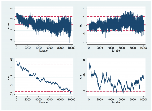
mcmcstats_v2 cons trt mon txm sd_r sd_p icc ,newey(100) ess
Convergence is still not perfect
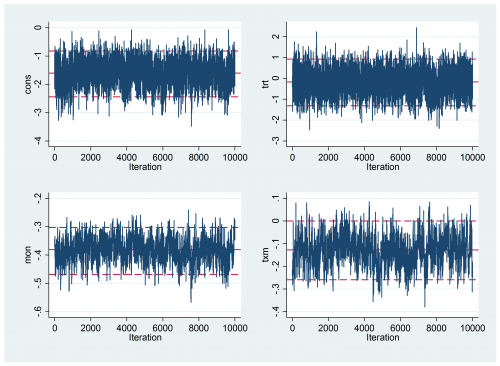
But it is much better than it was. The results are
-----------------------------------------------------------
 Parameter   n   mean    sd  ess  median     95% CrI
 ----------------------------------------------------------
 cons    10000 -1.614 0.424  679 -1.609 ( -2.450, -0.823 )
 trt     10000 -0.189 0.566 1334 -0.178 ( -1.322, 0.930 )
 mon     10000 -0.383 0.042  369 -0.382 ( -0.468, -0.303 )
 txm     10000 -0.129 0.067  328 -0.128 ( -0.259, 0.000 )
 sd_p    10000  3.946 0.357  165  3.936 ( 3.273, 4.679 )
 icc     10000  0.823 0.027  164  0.825 ( 0.765, 0.869 )
 ---------------------------------------------------------
Very similar to the results found by gllamm in Rabe-Hesketh and Skondal. We might get even closer agreement by weakening the prior on the patient variance and running a longer chain.
You might have noticed that this table includes ess, the effective sample size. I have been influenced my recent attempts to use MCMCglmm and Stan to add a couple of new options to mcmcstats including the effective sample size. I’ll discuss that another time.
As usual all of the programs referred in the posting can be downloaded from my webpage at https://www2.le.ac.uk/Members/trj and these include the version of mcmcstats that provided the effective sample size. Keep in mind that programs that I release as part of this blog are often under development and may change in the future.
There is quite a lot more to say about MCMCglmm; saving the random effect estimates, making predictions, analysing other type of model, more complicated variance structures etc. etc. I’ll return to this topic in the future but next week I want to start the process of explaining how Stan can be used with Stata. Stan is another stand-alone Bayesian analysis program but it takes a very different approach to WinBUGS and so opens up many new possibilities .

 Subscribe to John's posts
Recent Comments