
Last week I introduced the JAGS program as an alternative to WinBUGS and this week I started with the intention of comparing JAGS and WinBUGS using a sample dataset. I decided to base the comparison on the biopsy example taken from the WinBUGS help files.
Predictably, by the time that I had explained the model and fitted it by calling WinBUGS from Stata, I had already exceeded the quota of words that I allow myself each week, so I have split the posting in two. This week I will analyse the biopsy data in Stata by calling WinBUGS and next time I will make the comparison with JAGS.
The example: Heart Biopsies
These data are supplied with WinBUGS as one of its examples and come from an early study of biopsies taken from transplanted hearts. The data were originally analysed in,
Spiegelhalter DJ and Stovin PG
An analysis of repeated biopsies following cardiac transplantation.
Statistic in Medicine 1983 2(1):33-40
During the first year after a heart transplant, patients have regular biopsies to check for rejection. Biopsies are done under local anaesthetic and involve passing a wire through a vein until it reaches the heart. Once there, 4 or 5 tiny tissue samples are taken from different parts of the transplanted heart and later these are graded by a pathologist for cellular changes that are indicative of rejection. Rejection grading is usually done on a four point scale, none-mild-moderate-severe. A moderate or severe grade would probably lead to an adjustment of the patient’s immunosuppression treatment.
At the time of this particular study the practice was to take 3 biopsies but, for a few subjects only 2 usable samples were obtained. In all, the dataset contains grades for 2 or 3 biopsies from 157 hearts. A typical data entry might be (1,2,0,0) meaning that there were 3 biopsies taken from this heart and one biopsy was graded ‘none’ and two were graded ‘mild’.
Cellular changes related to rejection are not uniform across the heart and a serious concern is the false negative rate whereby a heart is being rejected but by chance the biopsies are all taken from healthy areas of tissue; several biopsies are taken at the same time in order to minimise this risk. The overall state of a heart is defined by the grade of its worst affected region (not the worst biopsy). So when three biopsies are taken from a ‘moderate’ heart, the results might be (mild,mild,moderate) or (mild,moderate,moderate) or even (none,mild,mild) if the ‘moderate’ region is missed.
A model for these data has two components, a set of probabilities p1, p2, p3, p4 representing the proportion of hearts that are none, mild, moderate or severe and a matrix of classification error probabilities, e[,], connecting the heart’s grade with the grade of a single biopsy.
Biopsy Grade Constraint
Grade of Heart None Mild Moderate Severe
none 1 0 0 0
mild e21 e22 0 0 e21+e22=1
moderate e31 e32 e33 0 e31+e32+e33=1
severe e41 e42 e43 e44 e41+e42+e43+e44=1
Obviously a heart that is mildly affected could never produce a severely affected biopsy, so there are constraints on the e’s and there are only six free parameters. We will make one further, rather strong, assumption, which is that the three biopsies are independent of one another given the overall grade of the heart. The under this model the probability of the data entry (1,2,0,0) is p2*3*e21*e222 + p3*3*e31*e322 + p4*3*e41*e422
It would be an interesting exercise to try and set meaningful priors on the p’s and the e’s but for the purposes of this exercise I will follow the WinBUGS manual and use flat Dirichlet priors over all of the sets of probabilities that must sum to one.
Here is the WinBUGS model file for this problem
model
{
for (i in 1:ns){
niops[i] <- sum(biopsies[i, ])
true[i] ~ dcat(p[])
biopsies[i, 1:4] ~ dmulti(error[true[i], ], nbiops[i])
}
error[2,1:2] ~ ddirch(prior[1:2])
error[3,1:3] ~ ddirch(prior[1:3])
error[4,1:4] ~ ddirch(prior[1:4])
p[1:4] ~ ddirch(prior[]);
}
In this program, ns=157, biopsies[157,4] is the data matrix, true[157] is the vector of actual (unobserved) heart grades, p[4] is the vector of heart grade probabilities for this population, error[4,4] is the matrix of biopsy grade probabilities conditional on the true heart grade and prior[4] is a matrix of prior parameters. Notice that WinBUGS uses the same priors for p[] and for each row of error[]. This only makes sense because flat priors are used for all of the sets of probabilities and prior[] is set to (1,1,1,1) in the data file.
Now let’s see how WinBUGS handles the structural zeros in the values of error[]. Specifying this matrix correctly is essential if the model is to fit. Part of error[] is structurally known and so needs to appear in the data file and part of error[] is to be estimated and so it also needs to appear in the initial values file. In each file the remaining part is replaced by a missing value, NA.
So in the data file we need
1 0 0 0
NA NA 0 0
NA NA NA 0
NA NA NA NA
The initial values must fill in the missing spaces and an obvious choice would be
NA NA NA NA
0.5 0.5 NA NA
0.333 0.333 0.333 NA
0.25 0.25 0.25 0.25
I copied and pasted the biopsy data from WinBUGS into a text file that I called biopsy.txt, I then used the wbsdecode command to read these data into Stata and I kept the 157×4 dataset in the form of 4 Stata variables that I called grade1, grade2, grade3 and grade4. These data were saved in a file called biopsy.dta. Here is the Stata code that does that job,
. wbsdecode using biopsy.txt , clear
. rename biopsies_# grade#
. keep grade*
. save biopsy.dta
Now we are in a position to write a Stata program for fitting the model using WinBUGS.
*———————————
* write data file
*———————————
use biopsy.dta, clear
matrix error = I(4)
forvalues r=2/4 {
forvalues c=1/4 {
if `c’ `r’ | `r’ == 1 matrix error[`r’,`c’] = .
else matrix error[`r’,`c’] = 1/`r’
}
}
wbslist (p=c(0.25,0.25,0.25,0.25)) (matrix error, format(%11.8f) ) ///
using init.txt , replace
*———————————
* write model file
*———————————
wbsmodel biopsy.do model.txt
/*
model
{
for (i in 1:ns){
nbiops[i] <- sum(biopsies[i, ])
true[i] ~ dcat(p[])
biopsies[i, 1:4] ~ dmulti(error[true[i], ], nbiops[i])
}
error[2,1:2] ~ ddirch(prior[1:2])
error[3,1:3] ~ ddirch(prior[1:3])
error[4,1:4] ~ ddirch(prior[1:4])
p[1:4] ~ ddirch(prior[])
}
*/
*———————————
* write script file
*———————————
wbsscript using script.txt , replace ///
model(model.txt) data(data.txt) init(init.txt) ///
log(log.txt) burnin(1000) update(10000) ///
set(error p) coda(bs)
*———————————
* run and read the results
*———————————
wbsrun using script.txt
type log.txt
wbscoda using bs , clear
*———————————
* inspect the results
*———————————
mcmcstats *
mcmctrace p*
Convergence is not a problem so I will only show the trace plots of p[].

Here are the results.
 -------------------------------------------------------------
 Parameter     n  mean    sd    sem median     95% CrI
 -------------------------------------------------------------
 error_2_1 10000 0.587 0.066 0.0013 0.588 ( 0.456, 0.714 )
 error_2_2 10000 0.413 0.066 0.0013 0.412 ( 0.286, 0.544 )
 error_3_1 10000 0.342 0.046 0.0007 0.340 ( 0.256, 0.436 )
 error_3_2 10000 0.037 0.018 0.0002 0.035 ( 0.010, 0.078 )
 error_3_3 10000 0.621 0.048 0.0007 0.622 ( 0.522, 0.711 )
 error_4_1 10000 0.099 0.042 0.0005 0.094 ( 0.034, 0.197 )
 error_4_2 10000 0.022 0.023 0.0003 0.015 ( 0.001, 0.086 )
 error_4_3 10000 0.204 0.061 0.0008 0.198 ( 0.101, 0.337 )
 error_4_4 10000 0.675 0.073 0.0010 0.679 ( 0.523, 0.804 )
 p_1       10000 0.153 0.050 0.0011 0.155 ( 0.049, 0.246 )
 p_2       10000 0.311 0.055 0.0010 0.307 ( 0.216, 0.432 )
 p_3       10000 0.389 0.044 0.0006 0.388 ( 0.305, 0.477 )
 p_4       10000 0.147 0.030 0.0003 0.145 ( 0.094, 0.211 )
 ---------------------------------------------------------------
The only problem is that I do not like the answer.
The estimates show that this population of hearts splits approximately; none 15%, mild 31%, moderate 39% and severe 15%. If the heart is truly in severe rejection there is a 68% chance that a biopsy will be graded as ‘severe’ and a 20% that it will be graded as ‘moderate’ and a 12% that it will be graded ‘none’ or ‘mild’, but ‘none’ is much more likely than ‘mild’.
For moderately rejected hearts there is a 62% of a ‘moderate’ biopsy and a 34% chance of a biopsy graded ‘none’ but almost no chance of a biopsy that is graded as ‘mild’.
It is estimated that about 1/3 of hearts show mild rejection, so it is not as though the mild category has been defined so narrowly that it is never seen in practice. These data give the picture of one or more regions of rejection with other regions with no rejection but nothing in between. In fact we hardly ever see mild biopsies unless the heart’s grade is mild.
It must be the case that,
• the mild category is truly a rare biopsy in a heart that is being rejected,
• something has gone wrong with the fitting,
• the model is wrong,
• we have not used our prior knowledge properly.
First we should look at the fit of the model but with discrete data of this type it is not obvious what scale we should use. In the end I decided to look at the average biopsy grade for each person and to contrast it with the predicted average under this model.
The average grade can be calculated from the data file as
. gen y = (grade1+2*grade2+3*grade3+4*grade4)/(grade1+grade2+grade3+grade4)
The predicted values of y, which I call ym, can be found by adding a couple of lines (shown in green) to the model file
model
{
for (i in 1:ns){
nbiops[i] <- sum(biopsies[i, ])
true[i] ~ dcat(p[])
biopsies[i, 1:4] ~ dmulti(error[true[i], ], nbiops[i])
y[i, 1:4] ~ dmulti(error[true[i], ], nbiops[i])
ym[i] <- (y[i,1]+2*y[i,2]+3*y[i,3]+4*y[i,4])/nbiops[i]
}
error[2,1:2] ~ ddirch(prior[1:2])
error[3,1:3] ~ ddirch(prior[1:3])
error[4,1:4] ~ ddirch(prior[1:4])
p[1:4] ~ ddirch(prior[])
}
Now we can use mcmccheck to create some residual plots. Here is the predictive distribution for heart 119 with the observation (none,mild,moderate) and an observed mean of (1+2+3)/3=2.
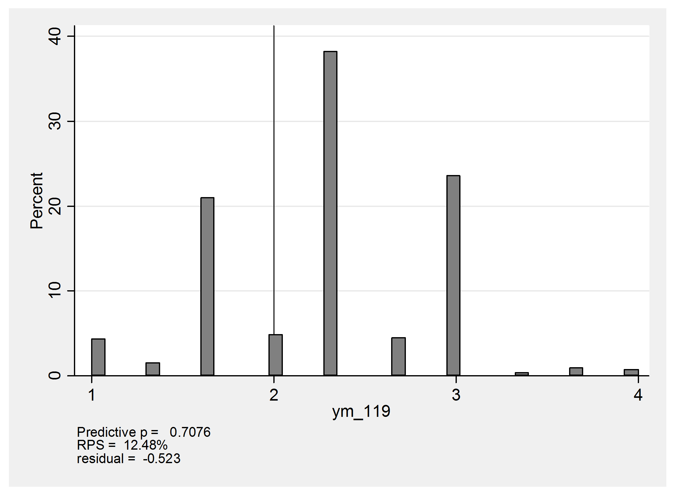
The predicted values of 1 arise from the possibility that this person is actually moderate or severe but the affected region is missed entirely and the biopsies are (none,none,none). The score of 4 would come about if the heart were actual severe, in which case there would be the chance that the biopsies would be graded (severe,severe,severe) instead of the observed (none,mild,moderate). In reality this heart has a mean score of 2 and falls just below expectation so that the standardized residual is about -0.5.
Here is the summary residual plot,
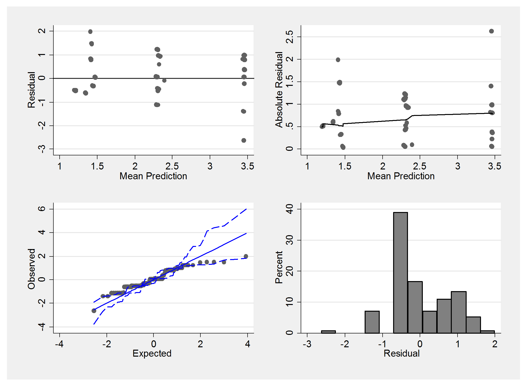
We must be careful not to judge these plots in the same way that we would the residuals from a linear model. The underlying scale is essentially discrete and so we would not expect normally distributed errors. Notice how the mean predictions suggest only 3 main groups with means falling between none and mild, mild and moderate and moderate and severe.
The extreme residuals in the summary plot come from people with grades such as (mild,mild,mild) and it could be that grades such as (mild,mild,mild) actually reflect a lack of independence in the sampling. Perhaps sometimes the biopsies are taken from the same region of the heart instead of spreading them around.
Here is a small simulation to show the impact of independence. Instead of sampling from an area I will sample from a line of length 1000. In the centre of this line is an affected region of length 200 which is graded as y=2, the remainder of the line has a grade of y=1. First we take two independent samples at random
set obs 1000
gen y = 1
replace y = 2 in 400/599
gen sample1 = .
gen sample2 = .
forvalues i = 1/1000 {
local j1 = int(runiform()*1000+1)
qui replace sample1 = y[`j1′] in `i’
local j2 = int(runiform()*1000+1)
qui replace sample2 = y[`j2′] in `i’
}
tabu sample1 sample2
Since a proportion 0.2 of the line is affected, we will obtain two affected samples with probability 0.2*0.2=0.04. The actual results vary slightly because of sampling error but here is a typical set that shows the anticipated pattern,
                    sample2
 sample1    |   1            2     | Total
 -----------+----------------------+----------
 1          | 638          182     | 820
 2          | 142           38     | 180
 -----------+----------------------+----------
 Total      | 780          220     | 1,000
Now change the sampling so that sample1 is chosen at random but sample 2 is taken within ±50 of sample1.
local j2 = max(min(`j1′ + int(runiform()*100+1)-50,1000),1)
Now a typical set of results is,
                   sample2
 sample1    |   1          2       | Total
 -----------+----------------------+----------
 1          | 758         26       |   784
 2          |  26        190       |   216
 -----------+----------------------+----------
 Total      | 784        216       | 1,000
Grade 2 still occurs about 20% of the time but clearly (2,2) and (1,1) have become much more common and (1,2) and (2,1) are much rarer. We could get the reverse effect if we were to insist that the two samples did not come from within ±50 of each other.
My suspicion is that for this particular data set, the assumption of independence of the sets of biopsies taken on the same occasion is an oversimplification. The oversimplified model will not predict the data very well and any attempt to interpret error[,] may be misleading.

 Subscribe to John's posts
Recent Comments