Solutions to the Exercises: Chapter 2

This is the second of my occasional postings working through the exercises given at the end of the chapters in ‘Bayesian analysis with Stata’. Chapter 2 was perhaps the most difficult chapter to write because I wanted to cover the creation of Stata programs for the calculation of the log posterior before I had introduced the simulation algorithms that make use of those programs. As a result some of the applications are a little artificial.

The exercises at the end of the chapter are relatively straight forward, none the less they raise some interesting issues. The code that is needed to analyse the examples is given in a separate downloadable pdf available here (chapter2 code) and in this posting I restrict myself to commenting on the answers and not the code. The questions, code and comments should really be viewed alongside one another.

Question 1

This question re-analyses some old data from an early breast cancer screening program. One of the trickiest aspects of the question is to assess your prior for the all-cause death rate per 100,000 women per year in unscreened women. The US Census Bureau data suggest a value around 600 deaths but there are uncertainties due to
• Not having national data for exactly the same years as HIPS
• Differences between HIPS and the National population both in geography and social class
• Uncertainty over the exact age structure of HIPS

In the end I opted for G(60,10) giving a mean on 600 (60×10) and a standard deviation of sqrt(60x10x10)=77, but of course you should rework the solution for your own priors and in a group exercise I would super-impose all of the priors on the same plot.

The downloadable code includes three ways of calculating the posterior.
• Using Stata’s integ command for numerical integration
• Using a program for calculating the log posterior
• Using the theoretical result that a Gamm distribution is conjugate for the Poisson mean
Of course, all three methods give the same result but the most generalizable approach is definitely the second of the three.

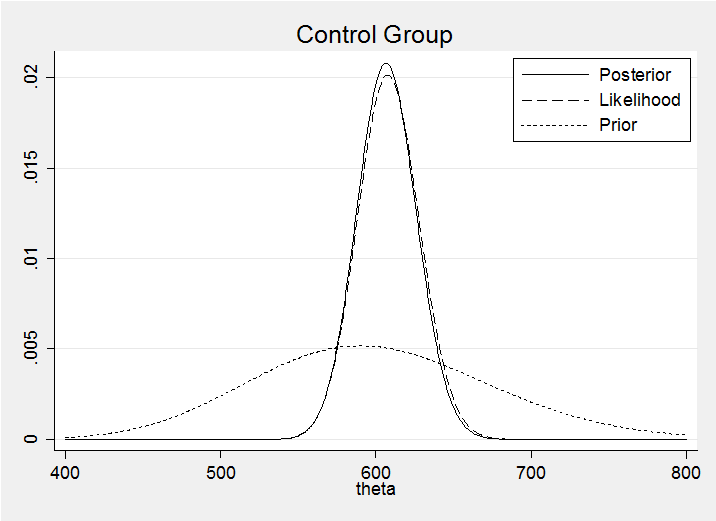
Here is the posterior superimposed on my prior and the likelihood normalized so that it displays conveniently on the same axes.

We can see that the prior has had little impact on the posterior. In a group exercise I would also superimpose all of the posteriors on the same plot in order to emphasise that the posteriors are much more similar than the priors.

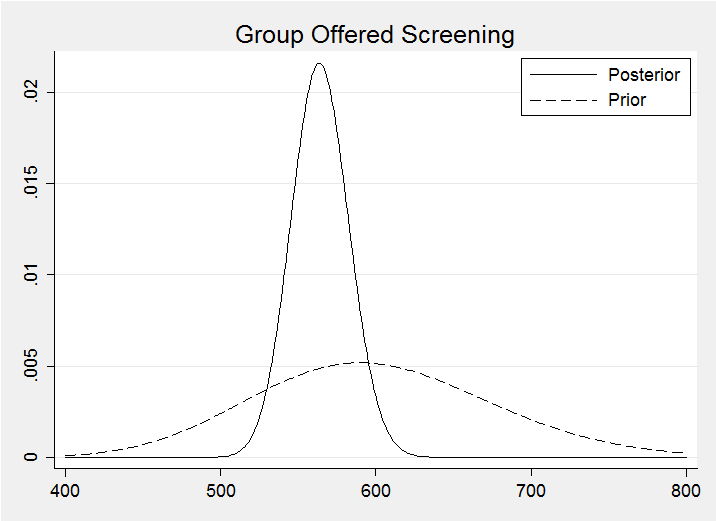
For the screened group I opted for a G(55,10) prior to reflect my belief that screening would be beneficial. My prior reduces the anticipated mortality by just under 10%. The method for calculating the corresponding posterior is identical to that used for the control group.

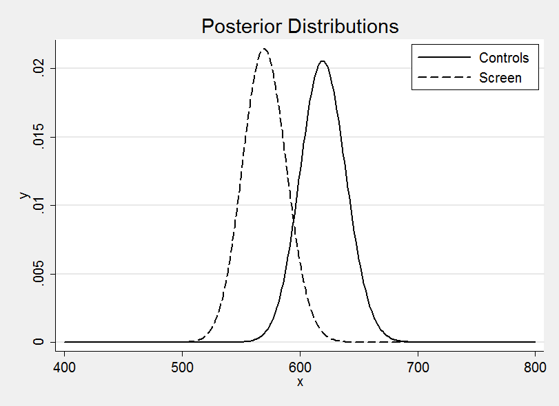
Plotting the two posterior distributions on the same graph suggests a benefit due to screening much as I anticipated.

It is interesting to distinguish two questions
(a) What is my best guess at the difference in mortality due to screening?
(b) Does HIPS provide evidence that screening makes a difference?
This analysis has addressed the first of these questions and the answer rightly depends on the HIPS study data plus everything else I believe about breast cancer screening. The second question is different and would require us to strip away my anticipated benefit and to consider only the evidence from the HIPS data. This can be done within a Bayesian context but it requires the calculation of a Bayes Factor and that is not covered until Chapter 10.

Is screening beneficial? – probably, but there are several reasons to hesitate
• The analysis conducted so far is influenced by my priors, which anticipated a difference? Perhaps we should conduct a sensitivity analysis with other priors
• The first few years of a screening program tend to pick up a backlog of late stage cancers that may be more difficult to treat – once established the screen should predominantly pick up early treatable cancers and show more benefit
• HIPS is not the whole world, so generalization is difficult – for instance, refusals might be much higher in another population and the benefit depends in part on the quality of treatment given to unscreened women.
• Remember that it is potentially misleading to assess a screening program based on cause-specific mortality, so don’t be tempted to base your assessment on the breast cancer deaths (imagine a type of mammogram that gave women lung cancer)

Question 2

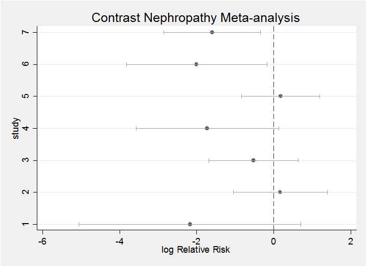
This question performs a meta-analysis of seven clinical trials. To give us a feel for the data here is forest plot based on frequentist estimates and confidence intervals.

The question requires us to start by setting a prior. My priors tend to be more informative than some people would be happy with (see my posting – Why I don’t use WinBUGS priors). In this case I felt that the treatment would do something between having no effect (log(1)=0) and halving the rate of contrast nephropathy (log(0.5)=-0.7). This led me to a rather conservative prior of N(-0.4,sd=0.3). We could also put priors on the sigma’s but as we only want a distribution conditional on knowing the sigma’s, there is no point.

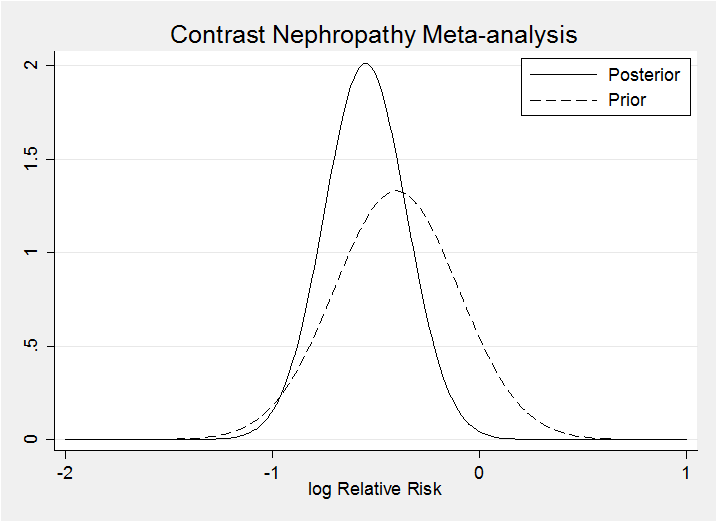
Calculation uses a program for calculating the log posterior and is shown in the pdf. My posterior and prior (dashed) for theta are

Clearly my prior is consistent with the data. Prior to seeing the data I gave a 9% chance that the drug would increase the risk of contrast nephropathy (lnRR>0) – after seeing the data this falls to 0.2%.

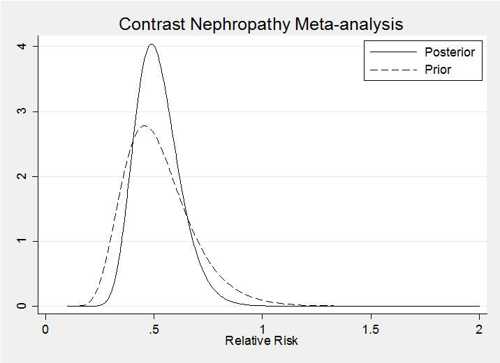
It is interesting to represent these distributions on the relative risk (RR) scale (note the Jacobian in the calculations)

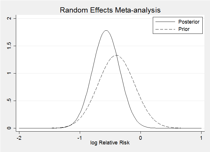
The result for the random effects model is very similar, at least when we condition on phi=0.5.

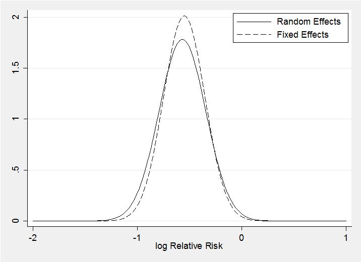
The random effects model makes little difference as the posteriors for theta under the two models demonstrate. The random effects posterior (solid line) is only slightly wider.

In this case it would be better to average over the distribution of phi and not to condition on a specific value but that requires the methods of chapter 3.