Monitoring Convergence in High Dimensions

In Chapter 5 of ‘Bayesian Analysis with Stata’ I discussed methods for monitoring the convergence of a set of MCMC simulations. Obviously it is important to demonstrate the effectiveness of different approaches to the assessment of convergence using output from real MCMC analyses, but often real problems are difficult to judge because we do not know the exact truth behind the convergence of the chain. What is more, with real chains it can be difficult to control the specific convergence characteristics that one wants to investigate.

An alternative way to judge a method for monitoring convergence is to use an artificial chain with a known structure and in the book I used artificially generated one-dimensional series to illustrate some of the standard methods for assessing convergence. It is relatively straight forward to generalize that approach into higher dimensions and I will discuss that approach here.

Our problem is to simulate an autocorrelated chain for a multidimensional set of parameters that together have a specified posterior distribution. A simple method for doing this is to make the target distribution a mixture of multivariate normals. We could generate the chain by running a chosen set of MCMC samplers with a specified target posterior that does not depend on any data, but in my method I simulate autocorrelated points directly from the target distribution.

For illustration, I ran a simulation of a chain of length 1000 with 3 parameters. In this case, the simulated posterior is composed of a single multivariate normal distribution with mean (5,5,5) and covariance matrix (2,2,2\2,3,3\2,3,4) but the chain starts with a poor initial guess of (4,10,0). The other feature that must be specified is the autocorrelation between sucessive points, which I set to be quite high at 0.95.

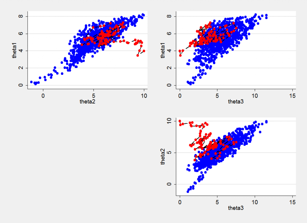
Here is a plot of the simulations. The first 100 points are shown in red and are joined in the order in which they were generated and the remainder, which represent the chain after the early drift, are shown in blue. We can see the impact of the poor initial values most clearly in the plot of theta2 against theta3.

The plot is also quite instructive in that it shows an unexpected blue tail of low values that was generated later in the chain. We are used to seeing random samples from a distribution in which occasional extreme values are generated but such extremes tend to be isolated. In a chain with high autocorrelation, one extreme value is likely to be followed by another. This is why highly correlated chains need to be run for so long even after they have recovered from the initial values.

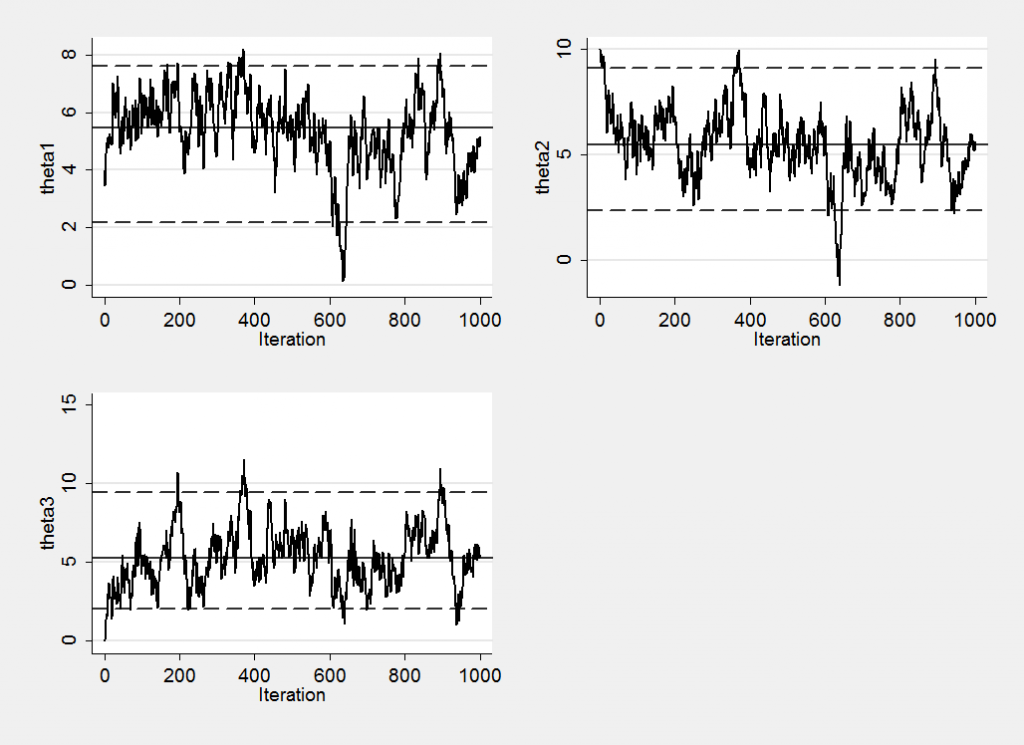
We might imagine that this early drift would be obvious in the marginal trace plots but in fact it is not that clear.

The early drift can be detected once we know that it is there and the blue tail is evident at around iteration 600, though not if we look at theta3. Using these trace plots alone, I doubt whether many people would have spotted the convergence problems.

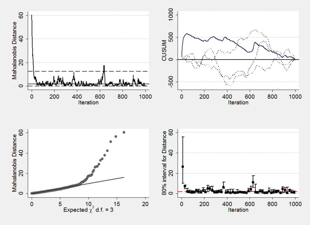
In the book I tried to stress the importance of thinking about convergence as a multi-dimensional issue and as an example of the type of methods that could be used I suggested plotting the Mahalanobis distance. This means plotting the Mahalanobis distance of the three dimensional points from the mean of the chain. The plot produced by mcmcmahal is,

I think that the features of the chain are clearer in this plot.

Next week I will return to this issue and say a little more about how my simulation program works and illustrate some convergence plots created from simulated posteriors with more complex shape. Meanwhile if you want to try these methods for yourself you can download the Stata code from here.