Model-free Genetic Meta-analysis

Some years ago some colleagues and I wrote a paper about the Bayesian meta-analysis of genetic association studies (Minelli et al Statistics in Medicine 2005;24:3845-3861) and periodically since then people have contacted me asking for the WinBUGS code that we used in that paper and those requests have prompted me to reformulate the code in terms of the functions for calling WinBUGS for Stata as described in the book ‘Bayesian Analysis with Stata’.

Here is the background to the paper although of course you can get more details from the original.

Many genetic studies relate a binary outcome (disease yes/no) to a specific genetic variant. Since our autosomal chromosomes occur in pairs, when a particular genetic variant can take one of two forms, say little a and big A, then that individual will we either aa, aA or AA (there is no way to distinguish aA from Aa). In effect then we have a 2×3 table of numbers of people.

	aa	aA	AA
Disease = Yes
Disease = No

We model these data in terms of the odds ratio of disease, but there are two odds ratios one for OR_aA = aA vs aa and one for OR_AA = AA vs aa. Very often researchers assume that OR_AA = OR_aA*OR_aA and for many diseases and variants this works well because it is like assuming that one’s risk increases equally with each extra copy of the A variant.

However, the assumption that OR_AA = OR_aA*OR_aA does not always apply and in the paper we suggested that we could use a meta-analysis to estimate both the form of the relationship between ORs and their sizes. We expressed the relationship in terms of a parameter

λ = logOR_aA/logOR_AA

What is more if we have an estimate of λ for a particular disease and variant, even if that estimate is subject to uncertainty, we can then use the information about OR_aA to improve our estimate of the OR_AA. Since a known or assumed relationship between OR_aA and OR_AA is called the mode of inheritance or sometimes the genetic model, we referred to our analysis as ‘genetic model free’.

We fitted this model using WinBUGS and investigated the impact of using different prior distributions using published and simulated data. Here I will show how we can automate such an investigation.

Let us start with some real data. Kato et al (Journal of Hypertension 1999;17:757-763) reported a meta-analysis of studies of a variant in the angiotensinogen gene and hypertension. Here is a summary of their data.

Study		Cases			Controls
	MM	TM	TT	MM	TM	TT
Hata, 1994	2	20	83	3	34	44
Iwai, 1994	3	17	62	4	30	49
Nishiuma, 1995	3	30	31	17	84	48
Morise, 1995	5	23	52	5	32	63
Sato, 1997	8	39	133	12	62	119
Kamitani, 1994	6	34	68	9	48	47
Kato, 1999	20	214	483	18	134	363

 

So here the two variants are labelled as M and T and in the first study 83 people with hypertension had the TT genotype. The key question is whether the T variant is more or less common in cases than in controls, with the genetic model being of secondary interest.

In the first study the researchers recruited 81 controls and found that they divided in the ratio 3:34:44. This we can model these data by a multinomial distribution with n=81 and probabilities p₀₁,p₀₂,p₀₃. We choose to parameterize β1=1, β2=p₀₂/p₀₁ and β3= p₀₃/p₀₁, then

p01=1/(1+ β2+ β3),    p02= β2/(1+ β2+ β3)    and     p03= β3/(1+ β2+ β3).

Similarly the 105 cases were in the ratio 2:20:83 and if these categories have probabilities q₀₁,q₀₂,q₀₃, we can parameterize them in terms of α1=1, α2=q₀₂/q₀₁ and α3= q₀₃/q₀₁. But α2/β2 is OR_TM and α3/β3 is OR_TT so we define δ2=logOR_TM and δ3=logOR_TT and the formulae for the probabilities in cases can be written,

q01=1/(1+ β2exp(δ2)+ β3 exp(δ3))

q02= β2exp(δ2)/(1+ β2exp(δ2)+ β3 exp(δ3))

q03= β3 exp(δ3)/(1+ β2exp(δ2)+ β3 exp(δ3))

Now the problem is parameterized in terms of β2, β3, δ2, δ3 and the genetic model as described by λ = δ2/δ3.

In a meta-analysis we would expect that β2, β3 could well be different for each study because genetic variants are sometimes more common in one population than another. Similarly δ3 might vary with population because frequently genes interact with aspects of the environment that differ between studies, however we might be willing to assume that the mode of inheritance, λ, is the same for all studies.

We treated the β’s as fixed effects, 2 for each study. δ3 as a random effect N(θ,τ²) and λ as a constant. A basic WinBUGS program for fitting this model is,

model {

       for( i in 1:7 ) {

              p[i,1] <- 1/(1+b[i,1]+b[i,2])

              p[i,2] <- b[i,1]/(1+b[i,1]+b[i,2])

              p[i,3] <- b[i,2]/(1+b[i,1]+b[i,2])

              q[i,1] <- 1/(1+b[i,1]*exp(lambda*d[i])+b[i,2]*exp(d[i]))

              q[i,2] <- b[i,1]*exp(lambda*d[i])/

                   (1+b[i,1]*exp(lambda*d[i])+b[i,2]*exp(d[i]))

              q[i,3] <- b[i,2]*exp(d[i])/

                   (1+b[i,1]*exp(lambda*d[i])+b[i,2]*exp(d[i]))

              d[i] ~ dnorm(theta,tau2)

              ncont[i,1:3] ~ dmulti(p[i,1:3],tcont[i])

              ncase[i,1:3] ~ dmulti(q[i,1:3],tcase[i])

              b[i,1] ~ dnorm(0,0.0001)

              b[i,2] ~ dnorm(0,0.0001)

       }

       lambda ~ dbeta(1,1)

       theta ~ dnorm(0,0.0001)

       tau2 ~ dgamma(0.001,0.001)

}

WinBUGS cannot fit this model and crashes but OpenBUGS runs it without a problem. Working within Stata we read the data from a file call kato.dta which has the same structure as the table shown above and variable names case1, case2 etc. Here is the entire code for fitting the model and viewing the results.

use kato.dta, clear

gen tcase = case1+case2+case3

gen tcont = control3+control2+control1

wbslist (struct case1 case2 case3 , name(ncase) format(%4.0f) ) ///

   (struct control1 control2 control3 , name(ncont) format(%4.0f) ) ///

   (vect tcase tcont) using data.txt, replace

matrix b=J(7,2,0.5)

wbslist (lambda=0.5,theta=0,tau2=1,d=c(7{0})) (matrix b , format(%4.1f)) ///

   using init.txt , replace

tomodel modelfree.do model.txt

/*

model {

       for( i in 1:7 ) {

              p[i,1] <- 1/(1+b[i,1]+b[i,2])

              p[i,2] <- b[i,1]/(1+b[i,1]+b[i,2])

              p[i,3] <- b[i,2]/(1+b[i,1]+b[i,2])

              q[i,1] <- 1/(1+b[i,1]*exp(lambda*d[i])+b[i,2]*exp(d[i]))

              q[i,2] <- b[i,1]*exp(lambda*d[i])/

                  (1+b[i,1]*exp(lambda*d[i])+b[i,2]*exp(d[i]))

              q[i,3] <- b[i,2]*exp(d[i])/

                   (1+b[i,1]*exp(lambda*d[i])+b[i,2]*exp(d[i]))

              d[i] ~ dnorm(theta,tau2)

              ncont[i,1:3] ~ dmulti(p[i,1:3],tcont[i])

              ncase[i,1:3] ~ dmulti(q[i,1:3],tcase[i])

              b[i,1] ~ dnorm(0,0.0001)

              b[i,2] ~ dnorm(0,0.0001)

       }

       lambda ~ dbeta(1,1)

       theta ~ dnorm(0,0.0001)

       tau2 ~ dgamma(0.001,0.001)

}

*/

wbsscript using script.txt, replace ///

       model(model.txt) data(data.txt) init(init.txt) log(log.txt) ///

       burnin(1000) update(10000) set(lambda theta tau2 b) ///

       coda(mf) openbugs

wbsrun using script.txt    , openbugs

wbscoda using mf , clear openbugs

gen OR3 = exp(theta)

gen OR2 = exp(lambda*theta)

gen sd = 1/sqrt(tau2)

mcmcstats *

and here are the results

--------------------------------------------------------------------------

Parameter         n     mean       sd     sem   median         95% CrI

--------------------------------------------------------------------------

 b_1_1       10000   18.437 11.803   0.7491   14.840 (   5.743, 51.549 )

 b_1_2       10000   28.600   18.929   1.7735   22.805 (   8.778, 83.620 )

 b_2_1       10000   11.348   5.987   0.2278   9.906 (   4.217, 27.469 )

 b_2_2       10000   20.655   11.225   0.6528   18.350 (   7.726, 50.830 )

 b_3_1       10000   6.615   1.868   0.0263   6.284 (   3.882, 11.079 )

 b_3_2       10000   3.879   1.185   0.0181   3.678 (   2.176,   6.757 )

 b_4_1       10000   7.459   3.066   0.0735   6.801 (   3.438, 15.370 )

 b_4_2       10000   14.312   6.138   0.1968   12.965 (   6.585, 30.110 )

 b_5_1       10000   5.798   1.577   0.0250   5.535 (   3.404,   9.478 )

 b_5_2       10000   11.550   3.170   0.0560   11.070 (   6.803, 19.010 )

 b_6_1       10000   6.534   2.117   0.0320   6.150 (   3.508, 11.730 )

 b_6_2       10000   6.929   2.412   0.0413   6.516 (   3.471, 12.870 )

 b_7_1       10000   9.813   1.793   0.0383   9.597 (   6.883, 13.910 )

 b_7_2       10000   24.927   5.075   0.1376   24.260 ( 16.790, 36.808 )

 lambda       10000   0.179   0.130   0.0025   0.155 (   0.007,   0.474 )

 tau2         10000   7.486   8.726   0.1713   5.117 (   0.887, 29.250 )

 theta       10000   0.541   0.252   0.0035   0.527 (   0.076,   1.083 )

 OR3         10000   1.775   0.502   0.0069   1.694 (   1.079,   2.954 )

 OR2         10000   1.117   0.135   0.0024   1.075 (   1.001,   1.465 )

 sd           10000   0.488   0.235   0.0042   0.442 (   0.185,   1.062 )

--------------------------------------------------------------------------

I will show a couple of convergence checks before commenting on these results.

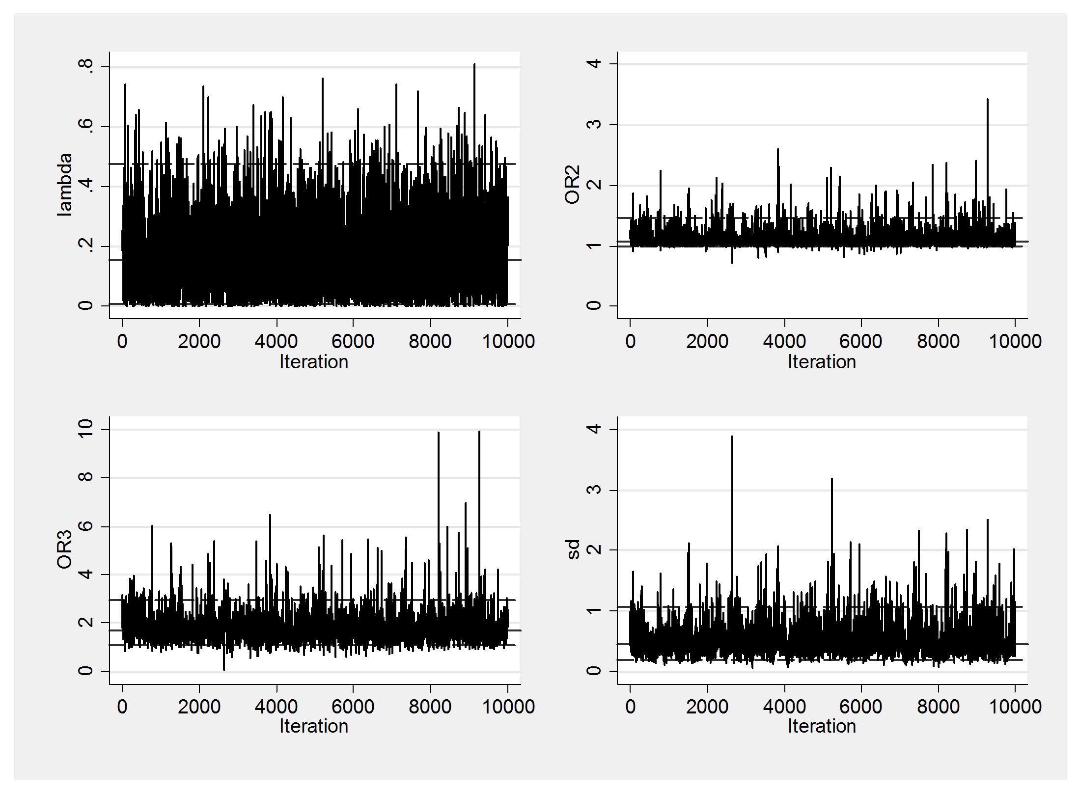
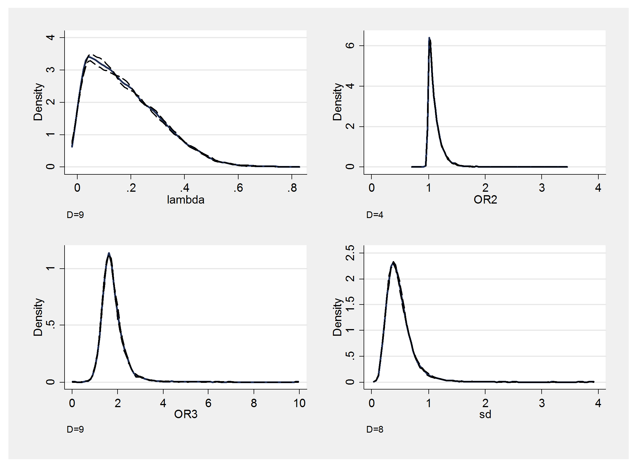
Mixing is fine and there is no obvious problem with the convergence, so let’s return to the findings.

The genetic model has an average lambda of about 0.18. On this scale 0.5 is the value that most people assume corresponding to OR_TT = OR_TM*OR_TM. This value is not well supported by the analysis and if anything we are closer to lambda=0 when OR_TM=1, which is known as the recessive model because we only see increased risk when both variants are T. Here the average effect of TT across the studies is to increase the odds of disease risk by 1.8 compared with MM individuals. The standard deviation is, however, quite large, which suggests that there is a lot of heterogeneity between studies. Perhaps, this variant interacts with something in the environment that differs across the populations or perhaps it is methodological, for instance it might relate to the inclusion criteria of the studies.

This particular analysis assumed a Beta distribution, B(1,1), for the prior on lambda this is flat between 0 and 1 but importantly excludes the possibility that lambda is outside that range. So this prior rules out the possibility the OR_TM> OR_TT. In the paper we looked at the impact of several different priors and I am sure that you can see other possibilities, such as assuming a fixed OR_TT or for putting structure on the betas.

In the paper we then simulated lots of datasets based on the pattern in the Kato study and investigated the fit. Suppose that we want to base our simulation on the posterior mean values of the betas,

use kato.dta, clear

gen tcase = case1+case2+case3

gen tcont = control3+control2+control1

input b1 b2

18.4 28.6

11.3 20.7

6.6 3.9

7.5 14.3

5.8 11.6

6.5 6.9

9.8 24.9

local lambda = 0.18

local sd = 0.49

local theta = 0.54

we can then simulate a new data set and write that to our data file

gen p1 = 1/(1+b1+b2)

gen p2 = b1/(1+b1+b2)

gen p3 = b2/(1+b1+b2)

gen d = rnormal(`theta’,`sd’)

gen OR2 = exp(d)

gen OR1 = exp(`lambda’*d)

gen q1 = 1/(1+b1*OR1+b2*OR2)

gen q2 = b1*OR1/(1+b1*OR1+b2*OR2)

gen q3 = b2*OR2/(1+b1*OR1+b2*OR2)

gen rcase1 = rbinomial(tcase,q1)

gen rcase2 = rbinomial(tcase-rcase1,q2/(q2+q3))

gen rcase3 = tcase-rcase1-rcase2

gen rcont1 = rbinomial(tcont,p1)

gen rcont2 = rbinomial(tcont-rcont1,p2/(p2+p3))

gen rcont3 = tcont-rcont1-rcont2

wbslist (struct rcase1 rcase2 rcase3 , name(ncase) format(%4.0f) ) ///

              (struct rcont1 rcont2 rcont3 , name(ncont) format(%4.0f) ) ///

              (vect tcase tcont) using data.txt, replace

This code creates a new dataset based on the Kato study and write it to the text file data.txt. We could place this code in a loop so that we generate lots of datasets and each time we could run OpenBUGS, read the results and store whatever we choose. Then we could run the do file and go and have tea, because it will take a while if we want a lot of simulations (we analysed 1,000 random datasets for each of several different choices of prior distribution).