Mixture Models: How many components?

In a recent posting I described a Stata program for Bayesian fitting of finite mixtures of multivariate normal distributions and I used it to smooth a histogram of fish lengths. The question that I would like to address now is, how do we control the amount of smoothing? If we employ very heavy smoothing then we will lose the distinct peaks and if the smoothing is too light our model will follow every random fluctuation in the histogram.

Non-Bayesians often select smoothing parameters by looking at the resulting curves and subjectively choosing one that looks reasonable. However, as Bayesians, we are used to setting priors before seeing the data and should not be drawn into this type of error. Instead we have two choices to make in advance of the analysis, both of which will affect the smoothing; first we must decide on the number of components to allow in the mixture and then we must choose our priors.

Selecting the Number of Components

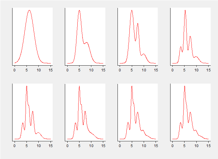
In a simple investigation I re-analysed the fish length data with different numbers of components but similar priors; all component means had N(6,sd=3.3) priors, the priors for the component precisions were G(1.5,1.5) and the Dirichlet prior on the mixture probabilities had alpha=(10,10,…) The plot below shows the average smoothed histogram for between 1 and 8 components.

By eye it appears that there is little to be gained in moving from 4 to 5 components, although from 5 onwards the fit does begin to capture the lack of symmetry in the main peak. The question is, how do we decide on the number of components before we see the data? There are two Bayesian strategies:

• Choose an unnecessarily large number of components and rely on the algorithm to make the probabilities of the unnecessary components very small. We might anticipate a small loss in precision in the smoothed histogram due to the uncertainty in the estimates of the redundant parameters, but at least we can be sure of having enough components. This approach leads naturally to the, so called, non-parametric Bayesian approach based on a mixture of an infinite number of normal distributions.
• Extend the analysis so that the number of components is a parameter in the model. Now the number is estimated based on the data plus the prior that we choose. Unfortunately this creates a new problem in that the algorithm for fitting the model needs to be able to cope with jumps between models with different numbers of parameters and this requires careful programming. A popular way of fitting such a model is to use a reversible jump algorithm.

These options will be good topics for future postings and eventually I hope to add programs for each of these to my library, libbayes.

Bayesians sometimes adopt an approach that is popular with frequentist statisticians, which is to define a measure of goodness of fit or accuracy of prediction and then to select the number of components that best fits the data according to that criterion.

I am not a fan of this approach, but it is simple to program and usually works well. My reservations are:

• The approach is essentially non-Bayesian as it is not based on the probabilities of different models.
• There is no obviously best measure of goodness of fit and different measures could suggest different numbers of components.
• We get no feel for the range of models that would have fitted almost as well as the best.

Perhaps the most widely used measure of the goodness of fit is the Bayesian Information Criterion (BIC), which despite its name is not a Bayesian measure. It is calculated as

-2 log-Likelihood + k log(n)

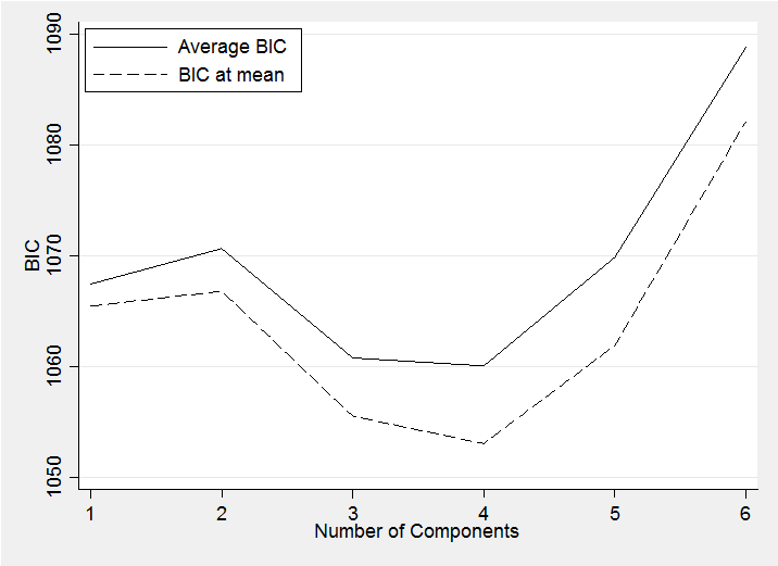
where the log-Likelihood is maximized over the model parameters and the penalty term involves k, the total number of parameters, and n, the number of observations. Bayesians do not maximize the log-Likelihood so cannot evaluate this BIC, instead they might calculate the BIC at the posterior mean estimates of the parameters (BIC at mean) or they might calculate the BIC at each iteration of the chain and then average (Average BIC). The results for these two approaches when applied to the fish data are shown are shown below.

Both curves confirm our visual impression that 5 is not better than 4 but the plot suggests that 3 components is better than 5 and I am not sure than I would accept that as I believe in the first small peak at around a length of 3 and this is not included in the 3 component model.

The difference between the two lines in this plot is approximately equal to the number of parameters; a fact that underlies the calculation of the Bayesian measure of fit known as the DIC.

Choosing the Priors

Let’s concentrate on the situation in which the individual components do not represent features that we know about in advance, because in that case we would use our knowledge to set different informative priors on each component. Rather let us suppose that all of the components are to have the same prior.

The prior on the mean of a component will be centred near the average of the data and its standard deviation will need to be large enough that each component’s mean could be anywhere within the range of the data. The fish lengths ranged up to about 12 inches and so I choose a mean of 6 and a standard deviation of just over 3. Other people might prefer something flatter over this range. It depends whether you expect that the component means will be evenly spread across the range.

The prior for the standard deviation of each component will, in part, be influenced by the number of components. If we think that there will be 4 main components and fish lengths range up to 12 inches then each component might be expected to cover about 3 inches and so have a standard deviation under 1 inch. There will be considerable uncertainty in this standard deviation but we would probably want a prior that discourages the standard deviation from being very small, so as to avoid producing a histogram with a large spike. I went for G(1.5,1.5) as the prior on the precision. This suggests that a precision is unlikely to be over 10 so that a standard deviation is unlikely to be below about 0.3.

Finally we need to set the Dirichlet prior on the probabilities of the components. If the parameter of the Dirichlet is alpha, then the expected proportion of the data that comes from the ith component is αi/Sum(αi) and very approximately its standard deviation is sqrt(αi)/Sum(αi) (the exact formula is given in the appendix to Bayesian analysis with Stata or you can find it in Wikipedia). So if we expect 4 large components and a couple of smaller ones then we might, for example set (5,5,5,5,1,1) or (10,10,10,10,2,2) etc. Under both options the first component is expected to contain 5/22=10/44=0.23 of the data. The approximate standard deviations would be either 0.10 or 0.07 suggesting proportions in the ranges (0.03 to 0.43) or (0.07,0.37).

What if you do not like the result?

I take a rather purist view about Bayesian analyses in that priors should not be modified based on the results of the analysis, so if your choices of the number of components and prior seem to over or under-smooth the distribution when you look at the results, then you have to live with it and put the poor choices down to experience.

In truth, if you have enough data to make you doubt the fit then only a grossly divergent prior would have any noticeable influence on the results. But a sensible precaution would be to simulate some datasets that follow a range of patterns that you could possibly see in the real data. If the results of analysing these data are not smooth enough then you can tweak the priors so that they better represent your true beliefs; but all this needs to be done before you analyse the real data.