
The Stata Journal has not published very much on Bayesian statistics, so I was delighted to see the article by Matthew Baker in the latest issue (Stata Journal 2014;14(3):623-661). Matthew describes a Mata program for adaptive MCMC and his paper has encouraged me to discuss this topic. You should certainly read that article alongside this blog.
I mentioned adaptation in chapter 3 of Bayesian analysis with Stata and I added an adapt option to the command –mcmcrun– so that users can automatically adapt the proposal standard deviations of their Metropolis-Hastings samplers. However, my approach was based on adaptation during the burn-in, while Matthew’s paper extends this approach to continued adaptation during the whole MCMC run. This is an interesting topic about which there has been quite a lot of research.
Adapting the sampler throughout the chain has the potential to be more efficient than fixing it at one value. Imagine sampling values from the conditional distribution of beta when the posterior resembles the plot below. Ideally we would like to use a proposal distribution for beta with a small standard deviation when alpha is around 10 but a proposal distribution with a much larger standard deviation when alpha is around 20. Since we are unlikely to have the information necessary for designing such a sampler when the chain starts, wouldn’t it be helpful if the chain could learn how to adapt the proposal distribution as it goes along?

A first sight adaptation looks attractive but before we start considering it, there is one very important message:
adapting the sampler during an MCMC run is dangerous.
So if you are not sure that it is valid, then don’t do it.
Beware the mathematician
In order for an MCMC algorithm to converge, we want the chain to have detailed balance, that is, it needs the property that for any two values of the parameter θ, say θ1 and θ2
P(θ1) P(move θ1 to θ2) = P(θ2) P(move θ2 to θ1)
Typically the moves are made dependent on (i) a proposal distribution and (ii) an acceptance probability, so the requirement for detailed balance becomes,
P(θ1) P(propose θ1 to θ2) P(accept θ1 to θ2) = P(θ2) P(propose θ2 to θ1) P(accept θ2 to θ1)
If we adapt the proposal distribution then we alter P(propose θ1 to θ2) as the chain progresses and we will have great difficulty in choosing an acceptance probability that ensures balance.
A simple solution to the problem is to insist that the changes to the proposal distribution get smaller over time; eventually they will fade away and the proposal distribution will almost be fixed and as a consequence we will eventually be able to choose acceptance probabilities that guarantee detailed balance. This is usually called diminishing adaptation.
Now there are mathematical proofs to the effect that if the changes in the proposal distribution fade towards zero then you can easily make the chain converge to the correct distribution. Unfortunately these are mathematical proofs about what will happen if the chain is run for ever and of course we do not run chains of infinite length.
Instead of accepting the mathematical proof, we must ask ourselves a more practical question. Suppose I run an adaptive chain for 10,000 iterations and maybe the proposal distribution is changed by noticeable, but diminishing amounts; will this have a meaningful impact on my estimated posterior distributions?
Remember that if we restrict adaptation to the discarded burn-in, as I do with the adapt option, then we will not have a problem.
A program for investigating adaptation
Here is a relatively general program for a random walk Metropolis-Hasting sampler that simulates values from a normal prior distribution with mean 1 and standard deviation 2. This may look rather unusual since we are used to simulating from posterior distributions that depend on data, while here we are simulating from a prior. It is also true that sampling from N(1,sigma=2) is trivial and does not need MCMC but there are advantages in testing an algorithm on a problem for which we know the correct answer.
To try to be clear, I will use sigma to represent the standard deviation of the target distribution and sd for the standard deviation of the proposal distribution.
 clear
 set seed 51817
 set obs 10000
 *----------------------------
 * INITIAL VALUES
 *----------------------------
 /*A*/ local sd = 1
 /*B*/ local lambda = 1
 gen sd = `sd'
 gen lambda = `lambda'
 gen theta = 1
 *----------------------------
 * 10,000 iterations
 *----------------------------
 local oldlogL = log(normalden(1,1,2))
 forvalues i=2/10000 {
 qui replace sd = `sd' in `i'
 qui replace lambda = `lambda' in `i'
 local j = `i' - 1
 *-------------------------------------
 * METROPOLIS-HASTINGS
 * & UPDATE PROPOSAL DISTRIBUTION (SD)
 *-------------------------------------
 local newtheta = theta[`j']+rnormal(0,`sd')
 local logL = log(normalden(`newtheta',1,2))
 if log(runiform()) < `logL' - `oldlogL' {
 qui replace theta = `newtheta' in `i'
 local oldlogL = `logL'
 local sd = `lambda'*`sd'
 }
 else {
 local sd = `sd'/`lambda'
 qui replace theta = theta[`j'] in `i'
 }
 *----------------------------
 * UPDATE DIMINISHING FACTOR
 *----------------------------
 /*C*/ local lambda = `lambda'
 qui replace lambda = `lambda' in `i'
 }
 histogram theta , ///
 addplot( function y = normalden(x,1,2), range(-5 7) ) ///
 leg(off)
 mcmcstats theta
 count if theta != theta[_n-1]
 mcmctrace theta lambda sd , cgopt(row(3))
I’ve highlighted 3 lines by labelling them as A, B and C. By changing those lines we can alter then properties of the algorithm.
The random walk updates have a standard deviation that is controlled by the local sd and the proposal distribution is altered by changing sd by an amount lambda. As the program stands, I set sd=1 and lambda=1 so the proposal distribution does not change. The mean posterior estimate of theta is 1.089 and its standard error (sem) is 0.0939. The standard deviation of the chain (estimating sigma) is 2.006. Here is a trace plot of the chain.
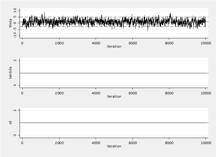
The chain mixes quite slowly because the proposal standard deviation is fixed at a value well below its optimal value. Setting line (A) to sd =4 produces better mixing with an estimate of 1.030 and a sem of 0.0422.
Both of these are valid chains that have detailed balance because sd is fixed. So now let’s allow sd to change and see what happens. If we return line (A) to read sd = 1 but put line (B) to lambda = 1.02. The proposal distribution will broaden when moves are accepted and narrow when a proposal is rejected. Eventually the chain will settle to reject about 50% of proposals. This is the algorithm used during the burn-in by –mcmcrun– whenever the adapt option is set.
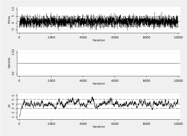
The proposal standard deviation moves quickly towards the (3,5) range. The mean of theta is 1.035 with a sem of 0.0416. The changes in the proposal distribution have no material impact the convergence. Sometimes sd is too large and sometimes it is too small but the effect is small and seems to cancel.
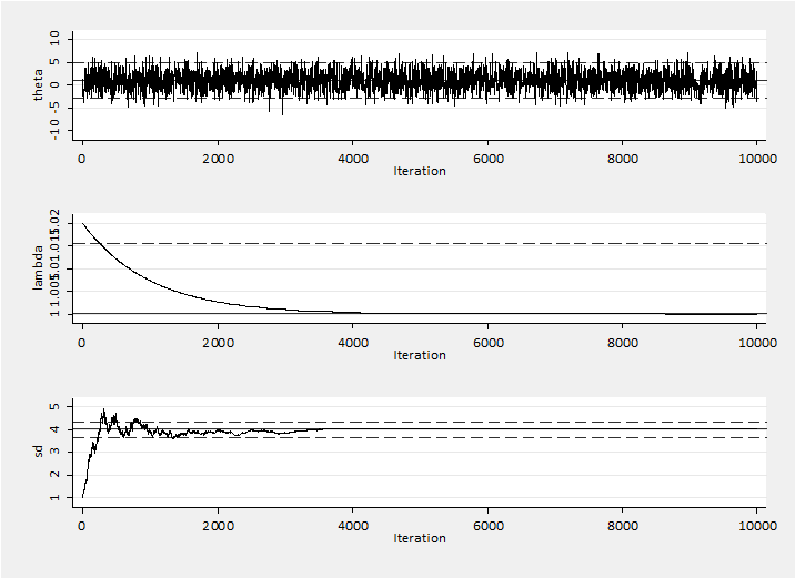
To create a diminishing effect we can set line (C) to be lambda = 1 + 0.02*0.999^`i’. Now we can see the impact of the diminishing changes in the way that sd settles around 4 once we pass iteration 4000 and lambda gets close to 1. The algorithm has the flexibility to adjust but we soon learn about the sd and the changes to become negligible. The results are fine with a posterior mean is 0.973 and sem=0.0414.
The difficulty with adaptation is that often we cannot be totally sure that the effect of the changes will be negligible within a run of finite length. This is especially true for problems with many correlated parameters, since the target conditional distribution will change depending on the values of the other parameters. For this reason I much prefer methods that adapt during the burn-in.
An Investigation
Here is a suggestion for an adaptive algorithm that you might like to try. Make the standard deviation of the proposal distribution equal to half the standard deviation of the previous m simulated values of the parameter. If sigma=2 then sd should have a mean of about 1. Start with m=50 and then investigate the effect of changing m. In this algorithm the adaptation does not diminish so you might also try allowing m to get larger as the chain increases in length.
Here is what happens if we set m to be fixed at 50.
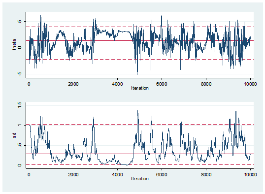
Clearly all is not well. Adaptive MCMC is potentially dangerous.

 Subscribe to John's posts
Recent Comments