Bayesian Experimental Design Part III

This week I am going to complete the discussion of Bayesian sample size calculation for a simple clinical trial. Here is the problem,

a trial is to compare a corticosteroid cream with a placebo for patients with eczema on their hand. The measurement of response will be the patient’s rating of the severity of their eczema on a 0-10 visual analogue scale (VAS). Patients will only be randomized if their baseline VAS is over 7 and success will be defined as a VAS below 3 after one week. How many patients do we need in the trial?

We suppose that the researcher believes that 50% of patients on the placebo will see enough improvement to be categorised as successful and the proportion of successes for the new drug will be around 70% but any level of success above 60% would be of clinical importance.

Two weeks ago we considered the sample size calculation based on the traditional power-based approach and I pointed out some of its limitations. Then in part II we considered the partial Bayesian solution based on the properties of the posterior of a measure of benefit. As part of that analysis, we elicited the researcher’s priors for p0, the probability of a successful outcome on placebo and the odds ratio θ=[p1/(1-p1)]/[p0/(1-p0)]. 70% success vs 50% translates into an odds ratio of 2.3 and 60% vs 50% is equivalent to an odds ratio of 1.5.

Now I want to create a full Bayesian solution incorporating utility and I want to implement it in Stata.

Full Bayesian analysis

The next discussion that we need to have with the researcher revolves around their reason for conducting the trial and how they will use the results. We need to establish the amount of information that the researcher really needs.

The chances are that the researcher wants to know whether or not the cream should be prescribed to future patients. Let’s suppose that they say that if the odds ratio, θ, really is over 1.5 then it will be worth recommending the treatment, while if θ<1.5, the cost of the cream will not justify its use. Of course, whatever the design of the experiment, the researcher will never know the true value of θ but rather they will have a posterior distribution for θ. So let’s suppose that the researcher says that they will recommend the cream if the posterior probability P(θ>1.5) exceeds 0.9.

This decision threshold acknowledges the possibility of making a mistake; either recommending the cream when really it has no benefit, or failing to recommend it when it would have been useful. These errors imply costs that can be contrasted with the benefits of reaching the right decision.

So we need to elicit the researcher’s costs and benefits, sometimes called their utilities. Let’s define the scale by saying that recommending the cream when it is really beneficial gives a utility of 1.0 and failing to recommend the cream when it is really useful gives a utility of zero.

	Recommend P(θ>1.5) exceeds 0.9	Fail to recommend P(θ>1.5) under 0.9
Beneficial True θ>1.5	Utility = 1.0	Utility = 0.0
Not Beneficial True θ <1.5

The researcher must use this scale to decide on the utility that they want to allocate when the cream is not truly beneficial. I’ll suppose that not recommending the cream when it is of no benefit is judged just as important as recommending it when it is beneficial, but that recommending it when it has no benefit is considered a serious error with a utility of -5.0

	Recommend P(θ>1.5) exceeds 0.9	Fail to recommend P(θ>1.5) under 0.9
Beneficial True θ>1.5	Utility = 1.0	Utility = 0.0
Not Beneficial True θ <1.5	Utility=-5.0	Utility=1.0

Now this very simple utility might not be sufficient. Perhaps the researcher would consider that recommending the cream when the true odds ratio is between 1.0 and 1.5 is not such a bad error but recommending it when the odds ratio is below 1.0 has a utility below even -5.0. We could expand the table into more categories, or even allow the utility to vary continuously with the true value of θ.

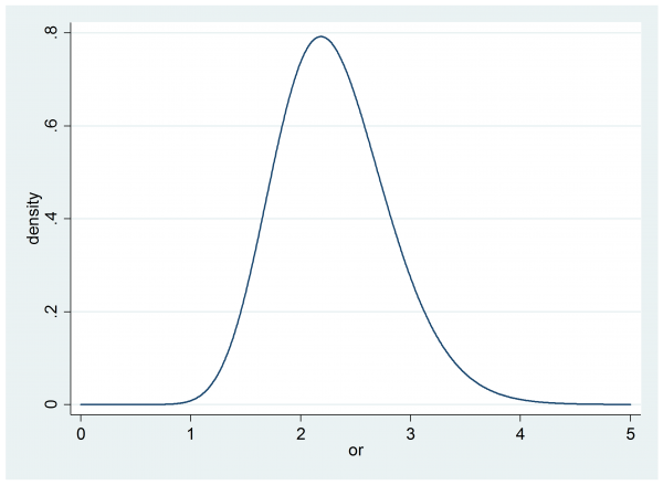
In part II we elicited the researcher’s prior for θ, it was gamma(20,0.115).

Before the trial there are no data, so this is effectively also the researcher’s posterior and we can calculate their probability that the odds ratio, θ, is over 1.5

. di 1- gammap(20,1.5/0.115)

This gives 0.956 or 95.6%. So prior to any trial, the researcher is more than 95% sure that the cream is beneficial and by their own decision rule, they would recommend the cream. In that case their expected utility is -5*0.044+1.0*0.956=0.736

It we collect data from a trial we would hope that if θ is truly less than 1.5 the posterior will move to the left and we will not recommend the cream, while if θ is greater than 1.5 the posterior will move to the right and narrow so that we will be even more likely to recommend the cream. Hopefully the utility will increase.

Indeed we could continue to recruit more and more subjects and eventually the posterior would just become a shape peak above the true value of θ. At that point we would never make a mistake and the expected utility would become 1.0. The balancing factor that stops us from an ever increasing sample size is the cost of adding extra subjects to the trial.

It is not easy to place the cost of recruiting an extra subject on the same scale as the utility of different decisions, but essentially that is what we do implicitly whenever we design a study. We ask ourselves, how do I balance the cost of the trial against the benefit of reaching the right conclusion? Only in most trials this balance is not quantified.

Often it helps to put our utilities into monetary terms. Perhaps we could consider the implications of the recommendation that we would make as a result of this trial and decide that a correct recommendation is worth £100,000. So that, in money, our utilities become

	Recommend P(θ>1.5) exceeds 0.9	Fail to recommend P(θ>1.5) under 0.9
Beneficial True θ>1.5	Utility = £100,000	Utility = £0.0
Not Beneficial True θ <1.5	Utility=-£500,000	Utility=£100,000

In money, under the researcher’s prior the expected gain from recommending the cream is £73,600 and the expected gain from not recommending the cream would be £100,000*0.044+£0*0.956=£4,400. So before any trial it is very clear to the researcher that they should recommend this cream.

Now let’s suppose that it costs £50 to recruit a patient.

An ideal trial that led to perfect recommendations would offer a benefit of £100,000. This is a gain of £26,400 over recommending the cream without running a trial. So we could recruit up to 26,400/50=528 patients into the trial and if the resulting trial improved our recommendations sufficiently then we would gain over not running a trial at all. However, given the researcher’s prior beliefs, it would never be sensible to recruit more than 528 patients. The hope is that between 0 patients and 528 patients we will find the best design.

Before embarking on a search for the best sample size, let’s try an arbitrary 75 patients in each arm of the study.

program logpost
    args lnf b

     local p0 = `b'[1,1]
     local or = `b'[1,2]
     local p1 = `or’*`p0’/(1-`p0’+`or’*`p0′)
     scalar `lnf’ = y0*log(`p0′)+(n-y0)*log(1-`p0′)+  y1*log(`p1′)+(n-y1)*log(1-`p1′) ///
          + 29*log(`p0′) + 29*log(1-`p0′) + 19*log(`or’) – `or’/0.115
end 

tempname pf
postfile `pf’ or pRec using utility.dta, replace
scalar n = 75
forvalues isim = 1/500 {
    local p0 = rbeta(30,30)
    local or = rgamma(20,0.115)
    local z = `or’*`p0’/(1-`p0′)
    local p1 = `z’/(1+`z’)
    scalar y0 = rbinomial(n,`p0′)
    scalar y1 = rbinomial(n,`p1′)
    matrix b = (0.5, 2.3)
    mcmcrun logpost b using temp.csv, replace ///
          samplers( (mhstrnc , sd(0.25) lb(0) ub(1) )  (mhslogn , sd(0.25) )  ) ///
          param(p0 theta) burn(500) update(2000)

    insheet using temp.csv, clear

    qui count if theta>=1.5
    local pRec = r(N)/2000
    post `pf’ (`or’) (`pRec’)
}
postclose `pf’
use utility.dta, clear
gen utility = 0
replace utility =  100000 if or >= 1.5 & pRec >= 0.9
replace utility =  100000 if or <  1.5 & pRec <  0.9
replace utility = -500000 if or <  1.5 & pRec >= 0.9
replace utility = utility-2*n*50
ci utility

In this program we simulate 500 sets of data under the researcher’s prior and we analyse those data and calculate the posterior probability that the odds ratio is over 1.5; I call this probability pRec since it is the probability on which we base the decision on whether to recommend the cream. Given the true value of the odds ratio, pRec and the sample size, n, we can calculate the expected utility.

In this case the results were,

Variable     |       Obs       Mean   Std. Err.       [95% Conf. Interval]
-------------+---------------------------------------------------------------
utility      |       500       69300   3949.014       61541.26   77058.74

Since not running the trial at all gave a return of £73,600 this appears to be worse than just using the cream and skipping the experiment, although the CI does not rule out a small gain so perhaps we need to run more than 500 simulations when calculating this expectation.

Of course if the trial were cheaper, say £25 per patient, then the total expected utility from a trial with 75 in each arm would be much closer to the return from not running an experiment and then we would certainly want to run more than 500 simulations in order to be able to assess whether the trial would be beneficial.

Having established the method for a trial of n=75 in each arm, we could repeat the calculation for a range of sample sizes and choose the best.

In this example I have supposed that the researcher was very sure beforehand that the cream would show a clinically important benefit, so it is not surprising that an experiment adds very little. The researcher might however argue that although I am convinced that the cream is beneficial, I need to run the trial in order to persuade others who are more sceptical. Here, we have an argument for using a different prior in the analysis to that used to generate the data.

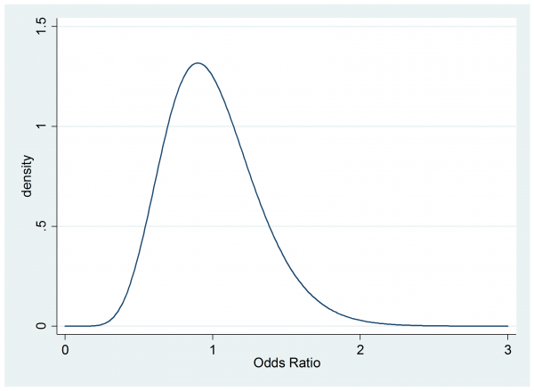
Suppose that a sceptical colleague has a prior for the odds ratio that is gamma(10,0.1)

. twoway function y=gammaden(10,0.1,0,x) , range(0 3) ytitle(density) xtitle(Odds Ratio)

This person believes that the cream might even be worse than the placebo and they think that the chance of a clinically important benefit (OR>1.5) is small so they would not recommend the cream without further evidence.

So if the researcher is right and the cream is actually highly beneficial the sceptic starts with an expected utility of 0.956*£0+0.044*£100,000 = £4,400 and a trial is much more likely to increase their utility.

To find how much their utility will increase, we merely re-run the program for the 500 simulations using the researcher’s prior for the data generation and the sceptical prior for the analysis. So the program for the log-posterior becomes,

program logpost 
    args lnf b

     local p0 = `b'[1,1]
     local or = `b'[1,2]
     local p1 = `or’*`p0’/(1-`p0’+`or’*`p0′)
     scalar `lnf’ = y0*log(`p0′)+(n-y0)*log(1-`p0′)+  y1*log(`p1′)+(n-y1)*log(1-`p1′) ///
          + 29*log(`p0′) + 29*log(1-`p0′) + 10*log(`or’) – `or’/0.1
end 

Here are the new results for n=75 in each arm of the trial.

Variable      | Obs Mean Std. Err. [95% Conf. Interval]
 -------------+---------------------------------------------
 utility      | 500 9800 1330.963 7185.018 12414.98

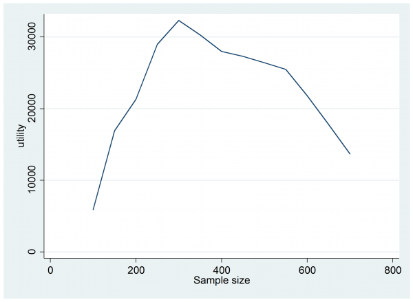
The expected utility has jumped from £4,400 to £9,800 so this trial would be worth doing, but perhaps a larger trial would be even more beneficial. Trial and error is probably sufficient to find the best design but I tried something a little more methodical by running 1,000 simulations for each sample size in the range n=200(50)700. Here is a plot of the results,

The design that offers the best expected return is a trial with 300 patients in each arm.

The program that created the last plot ran overnight; much more time consuming than the simple use of sampsi. Yet the biggest overhead is probably going to come from the elicitation of the priors and utilities, especially if the researcher is not used to this approach.

I hope that this example has demonstrated that the full Bayesian approach to design is much more realistic than a power based analysis and that it takes account of important factors that are simply ignored in a traditional sample size calculation. As so often happens, a Bayesian analysis makes explicit all of the assumptions that go into an analysis and as such the method can seem complex and even a little arbitrary. The truth is that those complicating factors do not go away when we run a non-Bayesian analysis, rather they are buried deep in the researcher’s judgement calls, such as their choice of the significance level and power.