Network Meta-analysis with WinBUGS and Stata

In my previous posting (https://staffblogs.le.ac.uk/bayeswithstata/2014/07/18/network-meta-analysis-in-stata/) I introduced an example of Network Meta-analysis taken from a NICE report that estimated the incidence of diabetes amongst people being treated for high blood pressure by one of six classes of drug. In that posting I analysed the data using Stata’s glm command and now I should like to analyse the same data using Stata and WinBUGS.

Programming the model in WinBUGS requires a little ingenuity because the trials do not include all of the treatments with some trials comparing two treatments and others comparing three. I will follow the NICE report in using d[1,…,6] to represent the treatment effects and mu[1,…,22] to represent study effects. Treatment 1 (diuretics) is chosen as the baseline, so d[1] is set to zero.

In the report vague priors are used throughout which negates one of the main benefits of a Bayesian analysis. However meta-analysis presents a particular problem for Bayesians because it is so difficult to produce informative priors that are not influenced, directly or indirectly, by the studies that we want to combine.

Once we have stacked the data as described in the previous posting, we can program the Bayesian analysis in Stata by preparing a do file as follows,

tomodel diabetes_fixed.do model.txt
/*
model{ 
   for(i in 1:48){ 
         r[i] ~ dbin(p[i],n[i]) 
         cloglog(p[i]) <- mu[id[i]]+d[t[i]]
   }
   d[1]<-0 
   for(k in 2:6){ d[k] ~ dnorm(0,0.0001) } 
   for(k in 1:22){ mu[k] ~ dnorm(0,0.0001) } 
}
*/
wbslist (vect id t r n , for("%6.0f")) using data.txt , replace
wbslist (mu=c(22{0}),d=c(NA,5{0})) using init.txt , replace 
wbsscript using script.txt , replace              ///
   model(model.txt) data(data.txt) init(init.txt) ///
   log(log.txt) coda(diab) burn(20000) update(20000) thin(2) set(mu d) dic
wbsrun using script.txt 
type log.txt
wbscoda using diab  , clear 
save diabetes_fit.dta, replace

mcmcstats d_2 d_3 d_4 d_5 d_6

–wbsmodel– is used to write the model to a text file (see my posting https://staffblogs.le.ac.uk/bayeswithstata/2014/03/21/keeping-good-records/  ). –wbslist– is used to write the data and initial values to a file. Notice how the first element of d is initialized to be missing (NA in WinBUGS) since it does not have a prior, but rather it has its value set to zero within the program.

The results calculated by WinBUGS are,

----------------------------------------------------------------------------

Parameter         n     mean       sd     sem   median         95% CrI

----------------------------------------------------------------------------

 d_2         10000   -0.247   0.057   0.0014   -0.247 ( -0.360, -0.133 )

 d_3         10000   -0.056   0.056   0.0017   -0.057 ( -0.163,   0.053 )

 d_4         10000   -0.253   0.053   0.0017   -0.254 ( -0.357, -0.148 )

 d_5         10000   -0.359   0.054   0.0013   -0.359 ( -0.464, -0.252 )

 d_6         10000   -0.453   0.063   0.0015   -0.452 ( -0.575, -0.330 )

----------------------------------------------------------------------------

For comparison here are the results from glm as reported in the previous posting

------------------------------------------------------------------------------

             |                 OIM

           r |     Coef.   Std. Err.     z   P>|z|     [95% Conf. Interval]

-------------+----------------------------------------------------------------

          2 | -.2469671   .0562828   -4.39   0.000   -.3572794   -.1366548

          3 |   -.056982   .0557689   -1.02   0.307   -.1662869     .052323

          4 | -.2530259   .0536676   -4.71   0.000   -.3582125   -.1478392

          5 |   -.358473  .0533383   -6.72   0.000   -.4630142   -.2539318

          6 | -.4527086   .0630479   -7.18   0.000   -.5762803   -.3291369

------------------------------------------------------------------------------

These are effectively equivalent as one would expect.

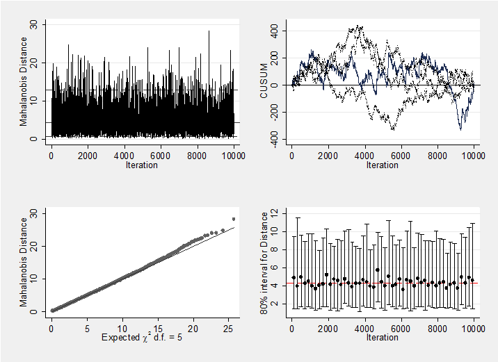
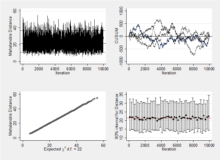
We should, of course, check convergence, but there does not seem to be a problem. For instance, the Geweke p-values for the 5 treatment effects are all non-significant (0.18, 0.19, 0.21, 0.10, 0.28 respectively). As a graphical summary, here are the mahalanobis plots for the 5 treatments differences and the 22 study effect. Neither indicates a problem with convergence.

mcmcmahal d_2 d_3 d_4 d_5 d_6

mcmcmahal mu_1-mu_22

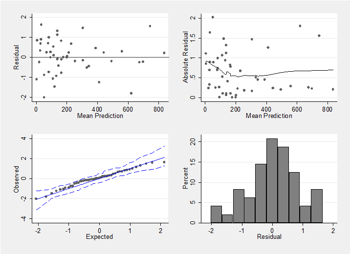
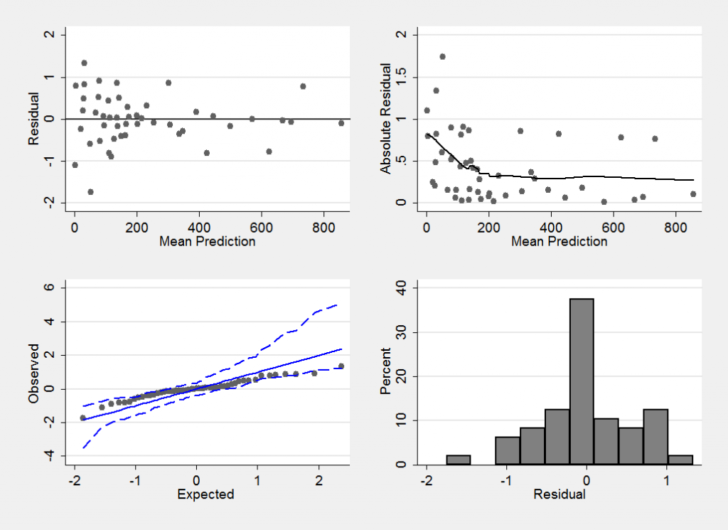
Convergence does not imply that we have a good model, so it makes sense to look at the residuals. When calculating the residuals the chain is thinned from length 20000 to length 1000 to avoid needlessly long calculations when constructing the residual plots.

I have chosen to calculate the residuals on the scale of r the number of cases of diabetes. In the model file below the vector f[] contains the predicted number of cases and these are read into Stata as f_1, f_2,…

wbsmodel diabetes_fixed.do modelf.txt
 /*
 model{
 for(i in 1:48){
 r[i] ~ dbin(p[i],n[i])
 cloglog(p[i]) <- mu[id[i]]+d[t[i]]
 f[i] ~ dbin(p[i],n[i])
 }
 d[1]<-0
 for(k in 2:6){ d[k] ~ dnorm(0,0.0001) }
 for(k in 1:22){ mu[k] ~ dnorm(0,0.0001) }
 }
 */
 wbsscript using script.txt , replace ///
 model(modelf.txt) data(data.txt) init(init.txt) ///
 log(log.txt) coda(diab) burn(20000) update(20000) ///
 thin(20) set(f)
 wbsrun using script.txt
 type log.txt
 wbscoda using diab , clear
 save pred.dta, replace

mcmccheck , dfile(stack_diabetes.dta) d(r) pfile(pred.dta) ///
 p(f_) plot(summary) save(diabetes_res.dta,replace)

This plot confirms that we have a reasonable model (perhaps the variability is slightly larger when fewer cases of diabetes are observed, but if so the effect is not strong).

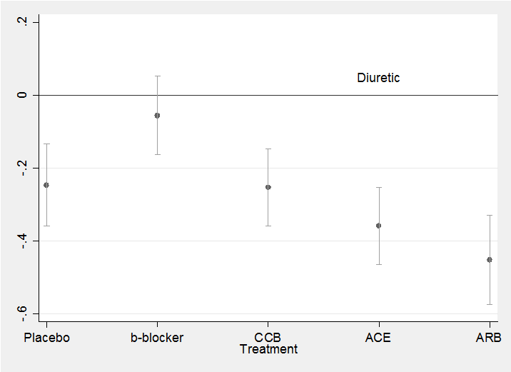
To plot the coefficients and their credible intervals as we did previously for the confidence intervals after the glm analysis,
use diabetes_fit.dta, clear
mcmcstats d_2 d_3 d_4 d_5 d_6 , save(est.dta,replace)
use est.dta, clear
gen id = _n
twoway (scatter mean id ) (rcap ub lb id ) , leg(off) ///
xlabel(1 “Placebo” 2 “b-blocker” 3 “CCB” 4 “ACE” 5 “ARB”) ///
yline(0) text(0.05 4 “Diuretic”) xtitle(Treatment)

In the NICE report the authors go on to fit a random effects model that allows the treatment effects to vary randomly by study. Here is a simplified model that is almost identical to the one used in the report.

model{ 
   for(i in 1:8){ 
         r[i] ~ dbin(p[i],n[i]) 
         e[i] <- 0
         cloglog(p[i]) <- mu[id[i]]+d[t[i]]
   }
   for(i in 9:48){ 
         r[i] ~ dbin(p[i],n[i]) 
         e[i] ~ dnorm(0,tau)
         cloglog(p[i]) <- mu[id[i]]+d[t[i]]+e[i]
   }
   d[1]<-0 
   for(k in 2:6){ d[k] ~ dnorm(0,0.0001) } 
   for(k in 1:22){ mu[k] ~ dnorm(0,0.0001) } 
   tau ~ dgamma(0.001,0.001)
}

A random effect e[] is added that allows the treatment effect d[] to vary randomly from study to study. The data are sorted so that the first 8 lines refer to trials in which subjects were treated with diuretics, that is to say with the baseline treatment. The DIC and parameter estimates for this model are almost identical to those given in the report for their model, which gives e[] a more compex variance structure.

The use of a random effects model reduces the DIC from 426 to 412, which by most guidelines would be considered as showing a better fit. In the report they certainly use this reduction to justify the random effects model. However if we look at the residuals we get a slightly different impression.

The residual are not as dispersed as we would expect under a binomial model and it looks to me like an example of over-fitting.

The DIC is widely used and almost as widely criticised. Its use has been questioned when we have a model with a large number of random effects and a small sample size. In this example there are 48 observations and the model with random effects has pD=37 suggesting the equivalent of 37 parameters. In this case I do not believe the DIC and I would use the earlier fixed effects model.

The WinBUGS code for the models recommended in the NICE report can be found at http://www.nicedsu.org.uk/TSD2%20General%20meta%20analysis%20corrected%2015April2014.pdf (the diabetes example starts on page 66). Those models can be fitted from within Stata using commands very similar to those given in the posting.