Network Meta-analysis in Stata

Regrettably clinical trials are often conducted that are too small to provide definitive evidence of the benefit of one treatment over another. In order to compensate for this, there has been a lot of work over the last twenty years on meta-analysing, or combining, the results from different trials. There is an example of a Bayesian meta-analysis in chapter 6 of the ‘Bayesian analysis with Stata’.

A complication that frequently arises in the meta-analyses of clinical trials is that different trials make slightly different treatments comparisons. So, in one trial a drug might be compared with a placebo and in another trial the same drug might be compared with an active control. Sorting out such a mixture of comparisons is often referred to as network meta-analysis.

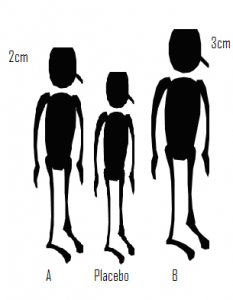
In a recent talk that I attended, the process of network meta-analysis was likened to measuring the height difference between three people. Let’s name the three people A, B and Placebo. In one experiment we compare A with Placebo and find that A in 2cm taller. Then in a separate study we compare B with Placebo and find that B is 3cm taller. Although we have never compared A and B directly we can deduce that B is taller than A by 1cm. The idea is simple but is it valid?

Suppose that subsequently we learn that the heights of A and Placebo were compared when they were both seated, while B and Placebo were compared when they were both standing. We can still calculate that the difference is 1cm but what does it represent? In fact the deduced difference has no useful meaning. You might assume that at least we know that B is the taller than A, but if it were the case that seated differences are always half those measured when standing, then A is actually taller than B.

One has to be very careful with analogies but we can easily see the consequences for treatments compared in clinical trials. Only when the trials comparing drug A with Placebo are conducted under exactly the same conditions as the trials comparing drug B with Placebo, can we be certain of obtaining a meaningful measure of the difference between A and B. Here, the ‘same conditions’ refers to anything that alters the measurement of treatment difference and might include factors such as, the inclusion/exclusion criteria, the exact form of the placebo treatment or the trial methodology; rarely will we be confident that these conditions are met.

Does the requirement for identical trial conditions matter? This is a difficult question to answer, certainly different conditions are likely to introduce bias into the indirect comparison of A and B but how big that bias will be will vary from problem to problem. There is however one sense in which this potential bias is very important. Organizations such as NICE (National Institute for Health and Care Excellence) in the UK have started to use network meta-analysis when considering which treatments to finance under the NHS (National Health Service) and a bias in such a comparison could have very important consequences.

For a much more detailed discussion of the assumptions needed for valid network meta-analysis see the recent articles by Donegan et al (Research Synthesis Methods 2013;4:291-323) and Jansen and Naci (BMC Medicine 2013;11:159).

There is a report that was produced for NICE that is a good starting point for anyone considering a Bayesian network meta-analysis as it contains a detailed review, followed by several examples together with the WinBUGS code required for their Bayesian analysis. ( http://www.nicedsu.org.uk/TSD2%20General%20meta%20analysis%20corrected%2015April2014.pdf  ).

One of the examples considered in the NICE report concerns a meta-analysis of the incidence of diabetes amongst people in trials of different treatments for hypertension. Concern is that the use of diuretics to treat high blood pressure might increase the risk of developing diabetes.

The report structures the data as,

+--------------------------------------------------------------------+

| time   t_1   r_1    n_1   t_2   r_2    n_2   t_3   r_3    n_3   na |

|--------------------------------------------------------------------|

|  5.8     1    43   1081     2    34   2213     3    37   1102    3 |

|  4.7     1    29    416     2    20    424     .     .      .    2 |

|    3     1   140   1631     2   118   1578     .     .      .    2 |

|  3.8     1    75   3272     3    86   3297     .     .      .    2 |

|    4     1   302   6766     4   154   3954     5   119   4096    3 |

|--------------------------------------------------------------------|

|    3     1   176   2511     4   136   2508     .     .      .    2 |

|  4.1     1   200   2826     5   138   2800     .     .      .    2 |

|    1     1     8    196     6     1    196     .     .      .    2 |

|  3.3     2   154   4870     4   177   4841     .     .      .    2 |

|    3     2   489   2646     5   449   2623     .     .      .    2 |

|--------------------------------------------------------------------|

|  4.5     2   155   2883     5   102   2837     .     .      .    2 |

|  4.8     2   399   3472     5   335   3432     .     .      .    2 |

|  3.1     2   202   2721     6   163   2715     .     .      .    2 |

|  3.7     2   115   2175     6    93   2167     .     .      .    2 |

|  3.8     3    70    405     4    32    202     5    45    410    3 |

|--------------------------------------------------------------------|

|    4     3    97   1960     4    95   1965     5    93   1970    3 |

|  5.5     3   799   7040     4   567   7072     .     .      .    2 |

|  4.5     3   251   5059     4   216   5095     .     .      .    2 |

|    4     3   665   8078     4   569   8098     .     .      .    2 |

|  6.1     3   380   5230     5   337   5183     .     .      .    2 |

|--------------------------------------------------------------------|

|  4.8     3   320   3979     6   242   4020     .     .      .    2 |

|  4.2     4   845   5074     6   690   5087     .     .      .    2 |

+--------------------------------------------------------------------+

So the first study compared three treatments (na=3) and followed its subjects for time=5.8 years. In that study, the treatments (t_1, t_2, t_3) were 1 (diuretics), 2 (placebo) and 3 (beta-blockers); 1081 (n_1) patients were treated with diuretics and of these 43 (r_1) were diagnosed with diabetes during the follow up period.

Bias might occur if, for example, diuretics tend to be compared with placebo in trials that recruit more elderly patients or perhaps more over-weight patients and if treatment differences are larger in such patients. Such unmeasured differences are a particular problem when they act multiplicatively.

A simple model for these data assumes a proportional hazards structure for the incidence of diabetes. This would imply that the probability, p, of developing diabetes in a follow up of length t years would be given by,
log(-log(1-p)) = Xβ + log H(t)
where H is the cumulative hazard and X is the design matrix. This complementary log-log transformation is commonly used for such data, although we have no way of confirming the proportional hazards assumption that underpins it.

Before embarking on the Bayesian analysis it is helpful to conduct a simple exploration of the data and to analyse them using maximum likelihood. This will give us a good indication of the answer that a Bayesian analysis would produce under non-informative priors.

A simple complementary log-log model is,
log(-log(1-pij)) = αi + δj + log Hi(ti)
where i denotes study and j denotes treatment. Since we have no information about the form of Hi we might as well combine that term with the study effects αi and write the model as
log(-log(1-pij)) = αi + δj

In the report the authors chose the model
log(-log(1-pij)) = αi + δj – δ1i + log(ti)
where δ1i is the first treatment applied in study i. This formulation is over-parameterized and makes it appear that we have information about the cumulative hazard that we cannot actually justify. The inclusion of δ1i changes the interpretation of the study effect but has no impact on the treatment differences. As the ordering of treatments within a trial is arbitrary it is hard to see why the authors chose to include δ1i. Probably this over-parameterization explains why the authors had to run their Bayesian analysis for so long before achieving convergence.

Let us consider a maximum likelihood analysis of the model,
rij ~ B(pij,nij)
log(-log(1-pij)) = μ + αi + δj
Under the constraint that α1=δ1=0
This is a standard generalized linear model that we can fit using the Stata command glm.

To fit the model we need to stack the data. So starting with the layout shown above,
gen id = _n
stack id time t_1 r_1 n_1 id time t_2 r_2 n_2 id time t_3 r_3 n_3 ///
, into( id time t r n) clear
drop if t == .
glm r i.id i.t, fam(bin n) link(cloglog)

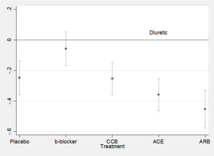
The estimates for the differences from treatment 1 (diuretics) are,

------------------------------------------------------------------------------

             |                 OIM

           r |      Coef.   Std. Err.      z    P>|z|     [95% Conf. Interval]

-------------+----------------------------------------------------------------

          2  |  -.2469671   .0562828    -4.39   0.000    -.3572794   -.1366548

          3  |   -.056982   .0557689    -1.02   0.307    -.1662869     .052323

          4  |  -.2530259   .0536676    -4.71   0.000    -.3582125   -.1478392

          5  |   -.358473   .0533383    -6.72   0.000    -.4630142   -.2539318

          6  |  -.4527086   .0630479    -7.18   0.000    -.5762803   -.3291369

------------------------------------------------------------------------------

Under proportional hazards, the coefficients represent log hazard ratios and so treatment 1 (diuretics) does have the highest rate of diabetes with all but treatment 3 (beta-blockers) showing a significantly lower rate.

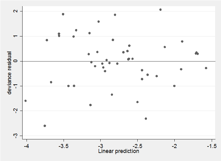
With any binomial analysis we need to be concerned about over-dispersion and in this case the Pearson X2/df ratio is 2.4 suggesting possible mild over-dispersion but nothing extreme. The deviance residual plot confirms this impression,
predict rd , deviance
predict xb , xb
scatter rd xb, yline(0)

The residuals show no pattern and most are within the range ±2 as we would hope. All in all, this simple model seems quite adequate to describe the data. We might neatly summarize the results in a plot of the treatment coefficients.

parmest , norestore
gen id = _n
twoway (scatter estimate id in 24/28) ///
(rcap min95 max95 id in 24/28) , leg(off) ///
xlabel(24 “Placebo” 25 “b-blocker” 26 “CCB” 27 “ACE” 28 “ARB”) ///
yline(0) text(0.05 27 “Diuretic”) xtitle(Treatment)

Anyone thinking of undertaking a Network Meta-analysis is Stata should visit the website
http://www.mtm.uoi.gr/index.php/stata-routines-for-network-meta-analysis
where they will find a collection of Stata programs for graphically representing networked trials. The recent Stata Journal article ‘Indirect treatment comparison’ by Miladinovic et al 2014:14(1)76-86 should also be of interest.

In my next posting I will return to the diabetes data and describe how we can combine Stata with WinBUGS to produce a Bayesian network meta-analysis of these data similar to that suggested in the NICE report.