Last time I started to discuss Bayesian experiment design and to illustrate that discussion I presented a simple clinical trial comparing a corticosteroid cream with a placebo for patients with eczema. The measurement of response was to be the patient’s rating of the severity of their eczema on a 0-10 visual analogue scale (VAS). Patients would only be randomized if their baseline VAS was over 7 and success was to be defined as a VAS below 3 after one week. I posed the question, how many patients do we need in the trial?
In discussing the traditional power-based calculation of sample size, I supposed that the researcher believed that 50% of patients on the placebo will see enough improvement to be categorised as successful and that the proportion of successes for the new drug would be 70%, but that any success rate over 60% would be of clinical importance.
The power-based sample size has many limitations so I went on to introduce a Bayesian algorithm based on the researcher’s prior for p0, the success probability under the placebo and p1, the success probability under the treatment.
Now I would like to see how this algorithm might be implemented in Stata.
Eliciting the priors
The basic parameters for this study are p0 and p1, but as we noted last time, beliefs about p1 and p0 are unlikely to be independent. So before we try to elicit priors for those probabilities directly, it is worth considering the alternatives.
We might start by considering the scale that will be used for measuring the benefit of treatment, which I will call θ. Possible options include, θ=p1-p0, θ=p1/p0, and θ=[p1/(1-p1)]/[p0/(1-p0)]. The first two have the advantage of simplicity but the disadvantage that there range depends on p0. So if p0 is 0.5 then θ=p1-p0 can lie in (-0.5,0.5), while if p0 is 0.3 then θ can lie in (-0.3,0.7). Were we to set priors on θ and p0 then we could not reasonably treat them as independent.
The odds ratio θ=[p1/(1-p1)]/[p0/(1-p0)] has the disadvantage of being harder to understand but the advantage that its range does not depend on p0 and so it is more reasonable to set independent priors on p0 and the odds ratio.
Our researcher said that their best guess was p0=0.5 and p1=0.7, which on the odds ratio scale implies θ=[0.7/0.3]/[0.5/0.5] = 2.3 and it turns out that p0=0.3 the p1=0.5 would give the same odds ratio θ=[0.5/0.5]/[0.3/0.7] = 2.3. So a key question is whether the researcher is happy that an improvement from 50% to 70% success is equivalent to a change from 30% to 50%.
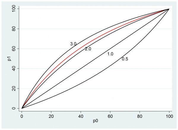
We might take a range of values of p0 and see what p1’s are implied by an odds ratio of 2.3 (the red line on the plot). The black lines show the relationships for other selected values of the odds ratio.
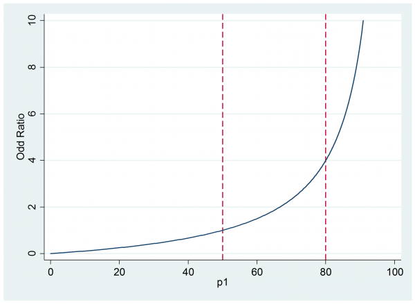
If this scale seems acceptable then we might present the researcher with a plot of the impact of different odds ratios when p0 is 0.5, as they expect.
Now they can judge that if the treatment is successful for between 50% and 80% of subjects then the implied odds ratio will be between 1 and 4.
Once you have explained the scale, the researcher will need to commit themselves to priors for p0 and θ. My preference is to let them sketch the priors freehand and then to try to find a standard distribution that is a reasonable approximation to their sketch.
Remember the old maxim that ‘all models are wrong, but some are useful’, well it is also true that ‘all priors are wrong, but some are useful’. So don’t be too particular about capturing those priors.
An alternative would be to get them to draw a histogram to represent the prior. For example, p0 could be described by a histogram with blocks that have a width of 0.05 or 5% depending on the units that they find easier. The histogram could itself be used as the prior or, as before, we could seek to approximate it by a standard distribution.
One advantage of finding a standard distribution is that one can select a distribution that does not totally rule out extreme values of the parameters. This is sometimes useful as values ruled out by the prior cannot be found in the posterior.
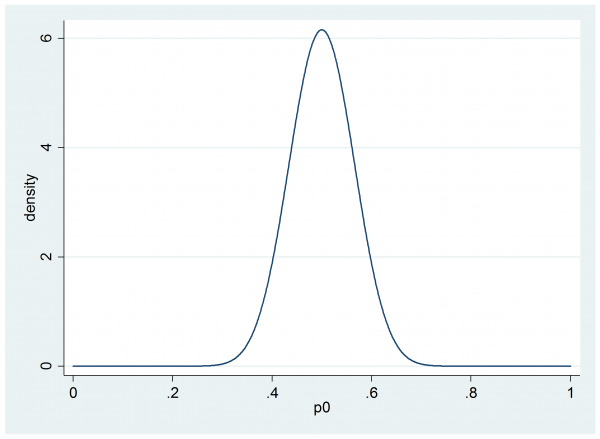
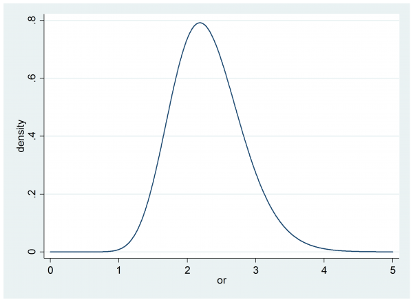
For illustration I am going to suppose that our researcher settles on a beta(30,30) prior for p0,
and an independent gamma(20,0.115). prior on the odds ratio, θ.
To continue working through the algorithm we need to define the criterion for selecting the best design. Here we have two options depending on whether the researcher is happy with a partial Bayesian solution in which they judge performance in terms of some measure associated with the posterior, or whether they want a full Bayesian design based on utility.
Partial Bayesian Design
Let’s start with the partial Bayesian design and suppose that the researcher is happy to measure performance in terms of the width of the 95% credible interval for the odds ratio. The more informative the experiment, the narrower will be this credible interval.
Before we collect any data, the 95% credible interval based on the researcher’s gamma prior can be calculated by the Stata commands,
. local lb = invgammap(20,0.025)*0.115
. local ub = invgammap(20,0.975)*0.115
so the interval is (1.405, 3.412) and has a width of almost exactly 2. The researcher must therefore tell us what width of credible interval they are hoping for once the trial is over. Perhaps they want to reduce the posterior width to 0.5.
Now we can simulate a random set of parameters from the priors and use them to simulate a data set of a chosen size. Let’s suppose that we decide to try a sample size of 100 in each group.
local p0 = rbeta(30,30)
local or = rgamma(20,0.115)
local z = `or’*`p0’/(1-`p0′)
local p1 = `z’/(1+`z’)
scalar y0 = rbinomial(100,`p0′)
scalar y1 = rbinomial(100,`p1′)
For illustration, I ran this once and got p0=0.50, or=1.96, p1=0.66 which led to y0=53 successes in the 100 placebo subjects and y1=59 successes in the 100 treated subjects. Now all we need to do is to calculate the posterior given these data and find the width of the posterior credible interval. Then we can repeat the simulation a few times to find the average or expected width and see if it is greater or less than the target. If n=100 proves too small or too large, we adjust the sample size and repeat until the expected width is close to 0.5.
So we need a program that calculates the posterior given data y0 and y1. The log-posterior is calculated by,
program logpost
args lnf b
local p0 = `b'[1,1]
local or = `b'[1,2]
local p1 = `or’*`p0’/(1-`p0’+`or’*`p0′)
scalar `lnf’ = y0*log(`p0′)+(100-y0)*log(1-`p0′)+y1*log(`p1′)+(100-y1)*log(1-`p1′) ///
+ 29*log(`p0′) + 29*log(1-`p0′) + 19*log(`or’) – `or’/0.115
end
Now we can find the expected width of the 95% credible interval. Since n=100 is likely to be a poor guess, I only ran the simulation and analysis 10 times.
tempname pf
postfile `pf’ w using width.dta, replace
forvalues sim = 1/10 {
drop _all
local p0 = rbeta(30,30)
local or = rgamma(20,0.115)
local z = `or’*`p0’/(1-`p0′)
local p1 = `z’/(1+`z’)
scalar y0 = rbinomial(100,`p0′)
scalar y1 = rbinomial(100,`p1′)
matrix b = (0.5, 2.3)
mcmcrun logpost b using temp.csv, replace ///
samplers( (mhstrnc , sd(0.25) lb(0) ub(1) ) (mhslogn , sd(0.25) ) ) ///
param(p0 theta) burn(500) update(2000)
insheet using temp.csv, clear
mcmcstats theta
local w = r(ub1)-r(lb1)
post `pf’ (`w’)
}
postclose `pf’
use width.dta, clear
ci w
The result was
    Variable |        Obs        Mean    Std. Err.       [95% Conf. Interval]
-------------+---------------------------------------------------------------
           w |         10     1.45993    .0581376        1.328413    1.591446
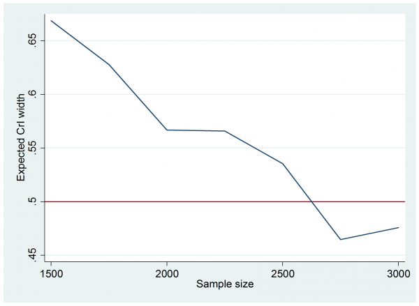
So the expected width is about 1.5 and 10 simulations were enough to place this expectation between 1.3 and 1.6. Since we are aiming for a width of 0.5 it is clear than n=100 is not nearly enough. A bit of trial and error followed and eventually I tried 25 simulations with each of the sample sizes in the range n=1500(250)3000. It only takes a couple of minutes to run.
The graph is not very smooth because I only ran 25 simulations at each sample size, none the less it is clear that we need around 2500 subjects in each group to get the 95% credible interval width down to 0.5.
This solution is almost certainly not practical and reflects the fact that we have based the design on an aspiration for a very precise experiment without considering the cost of the trial. We have also dodged the question of why the researcher wants so much accuracy.
Researchers naturally want to do highly informative experiments, but did our researcher really need to reduce the credible interval width to 0.5 or would 1.0 have been almost as useful? After all, they were expecting the odds ratio to be around 2.3, so a typical credible interval with width 0.5 would be (2.05,2.55), which is a very long way from what the researcher originally called a clinically important difference, p0=0.5 and p1=0.6, odds ratio 1.5.
As a postscript to the partial Bayesian analysis. I ought to mention the paper,
Wang F and Gelfand AE
A simulation-based approach to Bayesian sample size determination for performance under a given model and for separating models
Statistical Science 2002;17:193-208
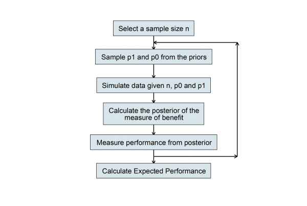
In this article the authors discuss the partial Bayesian solution based on the algorithm in the flowchart given earlier in this posting. The paper is especially useful because it considers many of the possible variations on this approach.
In their paper, Wang and Gelfand advocate using two prior distributions, one for sampling the data and a second for performing the analysis. This idea needs to be used with care as it produces an answer based on two contradictory assumptions. However, it can be useful. Imagine two people, A and B, who have different prior opinions. A asks the statistician, what sample size should I use in order to persuade B? This would require data simulated according to A’s prior and an analysis performed using B’s prior.
We will see an example of two priors in next week’s posting when I discuss the full Bayesian sample size calculation incorporating utility. That analysis will address the two issues of the precision that is actually required and the cost of the trial.


 Subscribe to John's posts
Recent Comments